Node classification: predictiong the label of a node in a graph. Link prediction: predicting the existence of an edge between two nodes. Graph classification: predicting the label of a graph.
Figure 1 illustrates these tasks.
Figure 1: Graph learning tasks. Courtesy of [1].
Figure 2 shows a representation of a node based on its neighbors.
Figure 2: node 5’s representation is updated based on its neighbors. Courtesy of [1].
In node classification node features + information from edges + information from the graph are represented.
Node representation
DeepWalk architecture is used to learn node representations. It is a two-step approach. First, it generates random walks (similar to a sequence of words) from the graph. Then, it uses SkipGram to learn the representations of the nodes.
Word2Vec (2013) uses NN to translate words into vectors. skip-gram predicts context words given a target word.
Assume n words: \(w_1, w_2, ..., w_N\). The goal is to maximize the probability of the context words given the target word. The probability is given by:
import numpy as np CONTEXT_SIZE =2 text ="""Lorem ipsum dolor sit amet, consecteturadipiscing elit. Nunc eu sem scelerisque, dictum erosaliquam, accumsan quam. Pellentesque tempus, lorem utsemper fermentum, ante turpis accumsan ex, sit ametultricies tortor erat quis nulla. Nunc consectetur ligulasit amet purus porttitor, vel tempus tortor scelerisque.Vestibulum ante ipsum primis in faucibus orci luctuset ultrices posuere cubilia curae; Quisque suscipitligula nec faucibus accumsan. Duis vulputate massa sitamet viverra hendrerit. Integer maximus quis sapien idconvallis. Donec elementum placerat ex laoreet gravida.Praesent quis enim facilisis, bibendum est nec, pharetraex. Etiam pharetra congue justo, eget imperdiet diamvarius non. Mauris dolor lectus, interdum in laoreetquis, faucibus vitae velit. Donec lacinia dui egetmaximus cursus. Class aptent taciti sociosqu ad litoratorquent per conubia nostra, per inceptos himenaeos.Vivamus tincidunt velit eget nisi ornare convallis.Pellentesque habitant morbi tristique senectus et netuset malesuada fames ac turpis egestas. Donec tristiqueultrices tortor at accumsan.""".split()
Code
skipgrams = []for i inrange(CONTEXT_SIZE, len(text) - CONTEXT_SIZE): array = [text[j] for j in np.arange(i - CONTEXT_SIZE,i + CONTEXT_SIZE +1) if j != i] skipgrams.append((text[i], array))print(skipgrams[0:3])
WARNING:gensim.models.word2vec:Both hierarchical softmax and negative sampling are activated. This is probably a mistake. You should set either 'hs=0' or 'negative=0' to disable one of them.
WARNING:gensim.models.word2vec:Both hierarchical softmax and negative sampling are activated. This is probably a mistake. You should set either 'hs=0' or 'negative=0' to disable one of them.
WARNING:gensim.models.word2vec:Effective 'alpha' higher than previous training cycles
Node embedding problem turn out to be foundational in graph machine learning tasks. We can use encoder and decoder perspective to learn node embeddings. Figures 3 and 4 illustrate the encoder and decoder perspective.
Figure 3: Encoder and decoder perspective. Courtesy of [2].
Here the goal is to learn an encoder that maps a node to a low-dimensional vector representation. The decoder is used to reconstruct the graph from the node embeddings.
\[ ENC: V \rightarrow R^d \]
\[ ENC(v_i) = z_i \]
\[ DEC: R^d \times R^d \rightarrow R^+ \]
\[ DEC(z_i, z_j) \approx S_{ij} \]
where \(z_i\) and \(z_j\) are the embeddings of nodes \(v_i\) and \(v_j\), respectively. \(S_{ij}\) is the actual similarity between nodes $ i and j$.
We can use the following loss function to train the encoder and decoder.
Figure 4: Encoder and decoder perspective. Courtesy of [2].
These type of node embeddings are shallow since node features are not used. Some of the shallow embedding methods are summarized in the following table.
Table 1: Summary of some of the shallow embedding algorithms. Courtesy of [2].
Node2Vec
Node2Vec (Grover, Leskovec, 2016) uses the main components of DeepWalk: random walk and Word2Vec. However, random walks are biased defining neighborhood based on BFS and DFS.
The transition probability from node \(v_i\) to \(v_j\) is given by:
where \(w_{ij}\) is the weight of the edge between \(v_i\) and \(v_j\). \(Z\) is the normalization constant. \(\alpha_{pq}(i,j)\) is the search bias. It is defined as:
where \(d_{ij}\) is the shortest path between \(v_i\) and \(v_j\). \(p\) and \(q\) are hyperparameters. \(p\) controls the likelihood of immediately revisiting a node in the walk. \(q\) controls the likelihood of exploring outward from the previous node. Greater q values result in exploring nodes close to the start no thus approximating BFS. Smaller q values result in exploring nodes further away from the start node thus approximating DFS.
Let’s implement Node2Vec using the python library.
A GNN is an optimizable transformation on all attributes of the graph (nodes, edges, global-context) that preserves graph symmetries (permutation invariances)[4].
In a basic neural network, input node A with features \(x_A\) is transformed with a weight matrix \(W\). The output is given by:
\[ h_A = \sigma(Wx_A) \]
where \(\sigma\) is the activation function.
In a GNN, the output of a node is a function of its neighbors. The output of node A is given by:
\[ h_A = \sigma(\sum_{B \in N(A)} Wx_B) \]
where \(N(A)\) is the set of neighbors of node A.
In matrix representation, a graph linear layer is given by:
\[ H = \hat A^T X W^T \]
where \(\hat A\) is the adjacency matrix with self-loops. \(X\) is the feature matrix. \(W\) is the weight matrix. Here is a sample code to implement a graph linear layer.
Code
import torch!pip install torch_geometricfrom torch_geometric.datasets import Planetoiddataset = Planetoid(root=".", name="Cora")from torch.nn import Linearimport torch.nn.functional as Fdata = dataset[0]def accuracy(y_pred, y_true):return torch.sum(y_pred == y_true) /len(y_true)class VanillaGNNLayer(torch.nn.Module):def__init__(self, dim_in, dim_out):super().__init__()self.linear = Linear(dim_in, dim_out, bias=False)def forward(self,x,adjacency): x =self.linear(x) x = torch.sparse.mm(adjacency, x) #multiplication with Areturn xfrom torch_geometric.utils import to_dense_adjadjacency = to_dense_adj(data.edge_index)[0] #edge index is coonverted to adjadjacency += torch.eye(len(adjacency)) #self loop addedclass VanillaGNN(torch.nn.Module):def__init__(self, dim_in, dim_h, dim_out):super().__init__()self.gnn1 = VanillaGNNLayer(dim_in, dim_h)self.gnn2 = VanillaGNNLayer(dim_h, dim_out)def forward(self, x, adjacency): h =self.gnn1(x, adjacency) h = torch.relu(h) h =self.gnn2(h, adjacency)return F.log_softmax(h, dim=1)def fit(self, data, epochs): criterion = torch.nn.CrossEntropyLoss() optimizer = torch.optim.Adam(self.parameters(), lr=0.01, weight_decay=5e-4)self.train()for epoch inrange(epochs+1): optimizer.zero_grad() out =self(data.x, adjacency) loss = criterion(out[data.train_mask],data.y[data.train_mask]) acc = accuracy(out[data.train_mask].argmax(dim=1), data.y[data.train_mask]) loss.backward() optimizer.step()if epoch %20==0: val_loss = criterion(out[data.val_mask],data.y[data.val_mask]) val_acc = accuracy(out[data.val_mask].argmax(dim=1), data.y[data.val_mask])print(f'Epoch {epoch:>3} | Train Loss:{loss:.3f} | Train Acc: {acc*100:>5.2f}% | Val Loss:{val_loss:.2f} | Val Acc: {val_acc*100:.2f}%')def test(self, data):self.eval() out =self(data.x, adjacency) acc = accuracy(out.argmax(dim=1)[data.test_mask], data.y[data.test_mask])return accgnn = VanillaGNN(dataset.num_features, 16, dataset.num_classes)print(gnn)gnn.fit(data, epochs=100)acc = gnn.test(data)print(f'\nGNN test accuracy: {acc*100:.2f}%')
zsh:1: command not found: pip
VanillaGNN(
  (gnn1): VanillaGNNLayer(
    (linear): Linear(in_features=1433, out_features=16, bias=False)
  )
  (gnn2): VanillaGNNLayer(
    (linear): Linear(in_features=16, out_features=7, bias=False)
  )
)
Epoch   0 | Train Loss:2.187 | Train Acc: 13.57% | Val Loss:2.24 | Val Acc: 9.40%
Epoch  20 | Train Loss:0.058 | Train Acc: 100.00% | Val Loss:1.48 | Val Acc: 74.40%
Epoch  40 | Train Loss:0.012 | Train Acc: 100.00% | Val Loss:1.96 | Val Acc: 74.40%
Epoch  60 | Train Loss:0.005 | Train Acc: 100.00% | Val Loss:2.05 | Val Acc: 74.40%
Epoch  80 | Train Loss:0.004 | Train Acc: 100.00% | Val Loss:2.06 | Val Acc: 74.40%
Epoch 100 | Train Loss:0.003 | Train Acc: 100.00% | Val Loss:2.04 | Val Acc: 74.80%

GNN test accuracy: 75.90%
Graph Convolutional Networks
Graph convolutional networks (GCNs) are a type of GNN. GNN did not take into account the difference in neighborhoods. GCNs apply a normalization that considers node degrees. GCNs are based on the convolution operation. A convolution layer with \(\hat D\) and \(\hat A\) is given by:
where \(H^{(l)}\) is the hidden state matrix at layer \(l\). \(W^{(l)}\) is the weight matrix at layer \(l\). \(\hat A\) is the adjacency matrix with self-loops. \(\hat D\) is the degree matrix with self-loops. \(\sigma\) is the activation function.
GCN(
  (gcn1): GCNConv(1433, 16)
  (gcn2): GCNConv(16, 7)
)
Epoch   0 | Train Loss:1.952 | Train Acc:  7.86% | Val Loss:1.95 | Val Acc: 8.40%
Epoch  20 | Train Loss:0.098 | Train Acc: 100.00% | Val Loss:0.79 | Val Acc: 77.00%
Epoch  40 | Train Loss:0.013 | Train Acc: 100.00% | Val Loss:0.75 | Val Acc: 77.80%
Epoch  60 | Train Loss:0.013 | Train Acc: 100.00% | Val Loss:0.73 | Val Acc: 77.80%
Epoch  80 | Train Loss:0.016 | Train Acc: 100.00% | Val Loss:0.72 | Val Acc: 77.80%
Epoch 100 | Train Loss:0.015 | Train Acc: 100.00% | Val Loss:0.73 | Val Acc: 78.00%
GCN test accuracy: 80.00%
GCN predictions: tensor([3, 4, 4,  ..., 1, 3, 3])
Graph Attention Networks
Graph attention networks (GATs) are a type of GNN. GATs use attention mechanism to learn the importance of neighbors. The attention mechanism is given by:
where \(x_i\) and \(x_j\) are the features of nodes \(i\) and \(j\), respectively. \(W\) is the weight matrix. \(||\) is the concatenation operator. \(\vec a\) is the attention vector. \(N(i)\) is the set of neighbors of node \(i\).
where \(\sigma\) is the activation function. Multiple attention heads are used to learn multiple representations of nodes. The output of node \(i\) is given by:
from torch_geometric.datasets import Planetoiddataset = Planetoid(root=".", name="Cora")data = dataset[0]import torchimport torch.nn.functional as Ffrom torch_geometric.nn import GATv2Convfrom torch.nn import Linear, Dropoutdef accuracy(y_pred, y_true):return torch.sum(y_pred == y_true) /len(y_true)class GAT(torch.nn.Module):def__init__(self, dim_in, dim_h, dim_out, heads=8):super().__init__()self.gat1 = GATv2Conv(dim_in, dim_h, heads=heads)self.gat2 = GATv2Conv(dim_h*heads, dim_out,heads=1)def forward(self, x, edge_index): h = F.dropout(x, p=0.6, training=self.training) h =self.gat1(h, edge_index) h = F.elu(h) h = F.dropout(h, p=0.6, training=self.training) h =self.gat2(h, edge_index)return F.log_softmax(h, dim=1)def fit(self, data, epochs): criterion = torch.nn.CrossEntropyLoss() optimizer = torch.optim.Adam(self.parameters(),lr=0.01, weight_decay=0.01)self.train()for epoch inrange(epochs+1): optimizer.zero_grad() out =self(data.x, data.edge_index) loss = criterion(out[data.train_mask],data.y[data.train_mask]) acc = accuracy(out[data.train_mask].argmax(dim=1), data.y[data.train_mask]) loss.backward() optimizer.step()if(epoch %20==0): val_loss = criterion(out[data.val_mask],data.y[data.val_mask]) val_acc = accuracy(out[data.val_mask].argmax(dim=1), data.y[data.val_mask])print(f'Epoch {epoch:>3} | Train Loss:{loss:.3f} | Train Acc: {acc*100:>5.2f}% | Val Loss:{val_loss:.2f} | Val Acc: {val_acc*100:.2f}%')@torch.no_grad()def test(self, data):self.eval() out =self(data.x, data.edge_index) acc = accuracy(out.argmax(dim=1)[data.test_mask], data.y[data.test_mask])return accgat = GAT(dataset.num_features, 32, dataset.num_classes)gat.fit(data, epochs=100)acc = gat.test(data)print(f'GAT test accuracy: {acc*100:.2f}%')
Epoch   0 | Train Loss:1.965 | Train Acc:  9.29% | Val Loss:1.94 | Val Acc: 15.20%
Epoch  20 | Train Loss:0.211 | Train Acc: 99.29% | Val Loss:0.94 | Val Acc: 72.20%
Epoch  40 | Train Loss:0.175 | Train Acc: 97.86% | Val Loss:0.88 | Val Acc: 73.00%
Epoch  60 | Train Loss:0.160 | Train Acc: 98.57% | Val Loss:0.90 | Val Acc: 73.60%
Epoch  80 | Train Loss:0.133 | Train Acc: 100.00% | Val Loss:0.93 | Val Acc: 71.00%
Epoch 100 | Train Loss:0.128 | Train Acc: 97.86% | Val Loss:0.92 | Val Acc: 74.40%
GAT test accuracy: 82.40%
GraphSAGE
GraphSAGE (Hamilton et al., 2017) is a type of GNN. GraphSAGE uses a neighborhood aggregation function to aggregate the features of a node’s neighbors. The neighborhood aggregation function is given by:
where \(h_i^{(l)}\) is the hidden state of node \(i\) at layer \(l\). \(W^l\) is the weight matrix at layer \(l\). \(\sigma\) is the activation function. \(AGG\) is the aggregation function. \(N(i)\) is the set of neighbors of node \(i\).
Figure 5 illustrates the GraphSAGE computation graph for a node.
Figure 5: Computation graph for node 0. Courtesy of [1].
GraphSAGE uses a sampling strategy to make the computation more efficient. The computation graph for node 0 is given in Figure 6.
Figure 6: Computation graph with sampling for node 0. Courtesy of [1].
GraphSAGE is an example of inductive learning. Inductive learning is the ability to generalize to unseen nodes.
Let’s implement GraphSAGE using PyG.
‘Inductive learning on protein-protein interactions. This dataset is a collection of 24 graphs, where nodes (21,557) are human proteins and edges (342,353) are physical interactions between proteins in a human cell. The goal of the dataset is to perform multi-label classification with 121 labels.’[1]
Code
!pip install torch_geometricfrom torch_geometric.datasets import PPItrain_dataset = PPI(root=".", split='train')val_dataset = PPI(root=".", split='val')test_dataset = PPI(root=".", split='test')print(len(train_dataset), len(val_dataset), len(test_dataset))train_dataset[19]#Unify training graph in a single set to apply neighbor samplingfrom torch_geometric.data import Batchfrom torch_geometric.loader import NeighborLoadertrain_data = Batch.from_data_list(train_dataset)loader = NeighborLoader(train_data, batch_size=2048,shuffle=True, num_neighbors=[20, 10], num_workers=2,persistent_workers=True)train_data[19]from torch_geometric.loader import DataLoadertrain_loader = DataLoader(train_dataset, batch_size=2)val_loader = DataLoader(val_dataset, batch_size=2)test_loader = DataLoader(test_dataset, batch_size=2)device = torch.device('cuda'if torch.cuda.is_available()else'cpu')from torch_geometric.nn import GraphSAGEmodel = GraphSAGE( in_channels=train_dataset.num_features, hidden_channels=512, num_layers=2, out_channels=train_dataset.num_classes,).to(device)criterion = torch.nn.BCEWithLogitsLoss()optimizer = torch.optim.Adam(model.parameters(),lr=0.005)def fit(): model.train() total_loss =0for data in train_loader: data = data.to(device) optimizer.zero_grad() out = model(data.x, data.edge_index) loss = criterion(out, data.y) total_loss += loss.item() * data.num_graphs loss.backward() optimizer.step()return total_loss /len(train_loader.dataset)from sklearn.metrics import f1_score@torch.no_grad()def test(loader): model.eval() data =next(iter(loader)) out = model(data.x.to(device), data.edge_index.to(device)) preds = (out >0).float().cpu() y, pred = data.y.numpy(), preds.numpy()return pred, f1_score(y, pred, average='micro') if pred.sum() >0else0for epoch inrange(301): loss = fit() preds, val_f1 = test(val_loader)if epoch %50==0:print(f'Epoch {epoch:>3} | Train Loss: {loss:.3f}| Val F1 score: {val_f1:.4f}')preds.shapepreds, test_f1 = test(test_loader)print(f'Test F1 score: {test_f1:.4f}')
zsh:1: command not found: pip
20 2 2
Epoch   0 | Train Loss: 0.590| Val F1 score: 0.4100
Epoch  50 | Train Loss: 0.190| Val F1 score: 0.8428
Epoch 100 | Train Loss: 0.142| Val F1 score: 0.8771
Epoch 150 | Train Loss: 0.122| Val F1 score: 0.8945
Epoch 200 | Train Loss: 0.107| Val F1 score: 0.9041
Epoch 250 | Train Loss: 0.097| Val F1 score: 0.9086
Epoch 300 | Train Loss: 0.090| Val F1 score: 0.9149
Test F1 score: 0.9351
Link Prediction
Link prediction is the task of predicting the existence of an edge between two nodes. Link prediction is used to recommend friends in social networks, recommend products in e-commerce, and recommend movies in streaming services.
We can distinguish between traditional link prediction and graph neural network-based link prediction.
Traditional link prediction methods are based on similarity measures. Common similarity measures are:
where \(A\) and \(B\) are the sets of neighbors of nodes \(i\) and \(j\), respectively. \(N(u)\) is the set of neighbors of node \(u\). \(walks(A,B,l)\) is the set of walks of length \(l\) between nodes \(A\) and \(B\). \(\beta\) is a hyperparameter.
Katz similarity calculation can be approximated using the following algebraic expression:
(I - \(\beta\)A)\(^{-1}\) - I
where \(I\) is the identity matrix. \(A\) is the adjacency matrix. Let’s implement these similarity measures.
Code
import networkx as nx# Create a simple graphG = nx.Graph()G.add_edges_from([(1, 2), (1, 3), (1, 4), (2, 3), (3, 4), (4, 5), (4, 6)])# Calculate Jaccard coefficient for potential new edgespotential_edges = []for u in G.nodes():for v in G.nodes():if u != v andnot G.has_edge(u, v): jaccard_coeff =len(list(nx.common_neighbors(G, u, v))) /len(set(G[u]) |set(G[v])) potential_edges.append((u, v, jaccard_coeff))# Sort potential edges by Jaccard coefficientpotential_edges =sorted(potential_edges, key=lambda x: x[2], reverse=True)# Predict links based on Jaccard's coefficientfor edge in potential_edges[:5]: # Predict top 5 edgesprint(f"Predicted edge between nodes {edge[0]} and {edge[1]} with Jaccard coefficient {edge[2]:.4f}")# networkx implementationpotential_edges = []for u, v in nx.non_edges(G): jaccard_coeff =len(list(nx.common_neighbors(G, u, v))) /len(set(G[u]) |set(G[v])) potential_edges.append((u, v, jaccard_coeff))print(potential_edges)
Predicted edge between nodes 5 and 6 with Jaccard coefficient 1.0000
Predicted edge between nodes 6 and 5 with Jaccard coefficient 1.0000
Predicted edge between nodes 2 and 4 with Jaccard coefficient 0.5000
Predicted edge between nodes 4 and 2 with Jaccard coefficient 0.5000
Predicted edge between nodes 1 and 5 with Jaccard coefficient 0.3333
[(1, 5, 0.3333333333333333), (1, 6, 0.3333333333333333), (2, 4, 0.5), (2, 5, 0.0), (2, 6, 0.0), (3, 5, 0.3333333333333333), (3, 6, 0.3333333333333333), (5, 6, 1.0)]
Code
import networkx as nximport math# Create a simple graphG = nx.Graph()G.add_edges_from([(1, 2), (1, 3), (1, 4), (2, 3), (3, 4), (4, 5), (4, 6)])# Calculate Adamic-Adar index for potential new edgespotential_edges = []for u in G.nodes():for v in G.nodes():if u != v andnot G.has_edge(u, v): adamic_adar =sum(1/ (math.log(G.degree(w))) for w in nx.common_neighbors(G, u, v)) potential_edges.append((u, v, adamic_adar))# Sort potential edges by Adamic-Adar indexpotential_edges =sorted(potential_edges, key=lambda x: x[2], reverse=True)# Predict links based on Adamic-Adar indexfor edge in potential_edges[:5]: # Predict top 5 edgesprint(f"Predicted edge between nodes {edge[0]} and {edge[1]} with Adamic-Adar index {edge[2]:.4f}")
Predicted edge between nodes 2 and 4 with Adamic-Adar index 1.8205
Predicted edge between nodes 4 and 2 with Adamic-Adar index 1.8205
Predicted edge between nodes 1 and 5 with Adamic-Adar index 0.7213
Predicted edge between nodes 1 and 6 with Adamic-Adar index 0.7213
Predicted edge between nodes 3 and 5 with Adamic-Adar index 0.7213
Code
import networkx as nximport numpy as np# Create a simple graphG = nx.Graph()G.add_edges_from([(1, 2), (1, 3), (1, 4), (2, 3), (3, 4), (4, 5), (4, 6)])# Get the mapping of nodes to indicesnode_to_index = {node: index for index, node inenumerate(G.nodes())}# Calculate Katz index for potential new edgesbeta =0.1# Adjust the beta value for the Katz indexadjacency_matrix = nx.to_numpy_array(G, nodelist=node_to_index.keys())I = np.identity(len(G.nodes()))katz_matrix = np.linalg.inv(I - beta * adjacency_matrix) - I# Calculate Katz index for potential new edgespotential_edges = []for u in G.nodes():for v in G.nodes():if u != v andnot G.has_edge(u, v): u_idx, v_idx = node_to_index[u], node_to_index[v] katz_index = katz_matrix[u_idx, v_idx] potential_edges.append((u, v, katz_index))# Sort potential edges by Katz indexpotential_edges =sorted(potential_edges, key=lambda x: x[2], reverse=True)# Predict links based on Katz indexfor edge in potential_edges[:5]: # Predict top 5 edgesprint(f"Predicted edge between nodes {edge[0]} and {edge[1]} with Katz index {edge[2]:.4f}")# playing with adjacency matrices to observe exponent relationship with number of walks of length limport numpy as np# Define the adjacency matrix for a simple graph with 6 nodes# Here, the matrix represents connections between nodes (1s for connections, 0s for no connections)A = np.array([ [0, 1, 1, 0, 0, 0], [1, 0, 1, 1, 0, 0], [1, 1, 0, 1, 1, 0], [0, 1, 1, 0, 1, 1], [0, 0, 1, 1, 0, 1], [0, 0, 0, 1, 1, 0]])# Calculate A^2 and A^3A_squared = np.dot(A, A)A_cubed = np.dot(A_squared, A)# Display the matricesprint("Adjacency Matrix A:")print(A)print("\nA^2 (A squared):")print(A_squared)print("\nA^3 (A cubed):")print(A_cubed)# Convert the adjacency matrix to a NetworkX graphG = nx.from_numpy_array(np.array(A))# Draw the graphnx.draw(G, with_labels=True)
Predicted edge between nodes 2 and 4 with Katz index 0.0237
Predicted edge between nodes 4 and 2 with Katz index 0.0237
Predicted edge between nodes 1 and 5 with Katz index 0.0119
Predicted edge between nodes 1 and 6 with Katz index 0.0119
Predicted edge between nodes 6 and 1 with Katz index 0.0119
Adjacency Matrix A:
[[0 1 1 0 0 0]
 [1 0 1 1 0 0]
 [1 1 0 1 1 0]
 [0 1 1 0 1 1]
 [0 0 1 1 0 1]
 [0 0 0 1 1 0]]

A^2 (A squared):
[[2 1 1 2 1 0]
 [1 3 2 1 2 1]
 [1 2 4 2 1 2]
 [2 1 2 4 2 1]
 [1 2 1 2 3 1]
 [0 1 2 1 1 2]]

A^3 (A cubed):
[[2 5 6 3 3 3]
 [5 4 7 8 4 3]
 [6 7 6 9 8 3]
 [3 8 9 6 7 6]
 [3 4 8 7 4 5]
 [3 3 3 6 5 2]]
These methods do not consider node features and structural similarity. They do not have inductive learning capability. Therefore, GNN-based link prediction methods are proposed.
Variational autoencoder for graphs (VGAE)
VGAEs learn normal distributions that are then sampled to produce embeddings. Encoder has two GCNs that share the first layer to 1. learn mean of latent normal distribution 2. learn variance of normal distribution Decoder samples embeddings z from the learned distributions. Inner product is used to approximate adjacency matrix.
zsh:1: command not found: pip
Epoch  0 | Loss: 3.5207 | Val AUC: 0.6133 | Val AP: 0.6447
Epoch 50 | Loss: 1.3293 | Val AUC: 0.6947 | Val AP: 0.7049
Epoch 100 | Loss: 1.1834 | Val AUC: 0.7303 | Val AP: 0.7335
Epoch 150 | Loss: 1.0535 | Val AUC: 0.7918 | Val AP: 0.7905
Epoch 200 | Loss: 1.0234 | Val AUC: 0.8266 | Val AP: 0.8192
Epoch 250 | Loss: 1.0053 | Val AUC: 0.8284 | Val AP: 0.8230
Epoch 300 | Loss: 0.9894 | Val AUC: 0.8306 | Val AP: 0.8257
Test AUC: 0.8359 | Test AP 0.8356
torch.Size([2708, 2708])
Subgraph based algorithms - SEAL
Enclosing subgraphs are extracted based on target nodes and their k-hop neighbors. Enclosing subgraph extraction, which consists of taking a set of real links and a set of fake links (negative sampling) to form the training data.Node information matrix construction, which involves three components – node labels, node embeddings, and node features.GNN training, which takes the node information matrices as input and outputs link likelihoods. Figure 7 illustrates the procedure.
Figure 7: SEAL steps. Courtesy of [1].
SEAL considers nodes labels determined based on the distances from target nodes. That is Double-radius node labeling (d(i,x), d(i,y)). The label for a neighbor node \(i\) is given by:
\[f(i)=1+min(d(i,x),d(i,y))+(d/2)[(d/2)+(d\%2)-1]\] where (d/2) and (d%2) are the quotient and remainder of d/2, respectively.
Optional node embeddings can be calculated using another algorithm, such as Node2Vec. Then, they are concatenated with the node features and one-hot encoded labels to build the final node information matrix.
The original SEAL algorithm is based on GCN - named deep graph convolutional neural network. Several GCN layers compute node embeddings that are then concatenated. A global sort pooling layer sorts these embeddings in a consistent order before feeding them into convolutional layers. Traditional convolutional and dense layers are applied to the sorted graph representations and output a link probability.
zsh:1: command not found: pip
Epoch  0 | Loss: 0.7031 | Val AUC: 0.6922 | Val AP: 0.6855
Epoch  1 | Loss: 0.6411 | Val AUC: 0.7725 | Val AP: 0.8044
Epoch  2 | Loss: 0.6129 | Val AUC: 0.7728 | Val AP: 0.8105
Epoch  3 | Loss: 0.6069 | Val AUC: 0.7729 | Val AP: 0.8136
Epoch  4 | Loss: 0.6047 | Val AUC: 0.7676 | Val AP: 0.8070
Epoch  5 | Loss: 0.6033 | Val AUC: 0.7680 | Val AP: 0.8097
Epoch  6 | Loss: 0.6015 | Val AUC: 0.7687 | Val AP: 0.8028
Epoch  7 | Loss: 0.6005 | Val AUC: 0.7653 | Val AP: 0.8002
Epoch  8 | Loss: 0.5980 | Val AUC: 0.7679 | Val AP: 0.7949
Epoch  9 | Loss: 0.5985 | Val AUC: 0.7673 | Val AP: 0.7957
Epoch 10 | Loss: 0.5973 | Val AUC: 0.7678 | Val AP: 0.7980
Epoch 11 | Loss: 0.5966 | Val AUC: 0.7654 | Val AP: 0.7973
Epoch 12 | Loss: 0.5960 | Val AUC: 0.7663 | Val AP: 0.7996
Epoch 13 | Loss: 0.5955 | Val AUC: 0.7659 | Val AP: 0.7977
Epoch 14 | Loss: 0.5943 | Val AUC: 0.7688 | Val AP: 0.8001
Epoch 15 | Loss: 0.5942 | Val AUC: 0.7696 | Val AP: 0.8046
Epoch 16 | Loss: 0.5929 | Val AUC: 0.7620 | Val AP: 0.7848
Epoch 17 | Loss: 0.5938 | Val AUC: 0.7702 | Val AP: 0.8010
Epoch 18 | Loss: 0.5921 | Val AUC: 0.7630 | Val AP: 0.7865
Epoch 19 | Loss: 0.5931 | Val AUC: 0.7671 | Val AP: 0.7988
Epoch 20 | Loss: 0.5916 | Val AUC: 0.7692 | Val AP: 0.8046
Epoch 21 | Loss: 0.5923 | Val AUC: 0.7674 | Val AP: 0.7917
Epoch 22 | Loss: 0.5915 | Val AUC: 0.7655 | Val AP: 0.7962
Epoch 23 | Loss: 0.5908 | Val AUC: 0.7669 | Val AP: 0.7937
Epoch 24 | Loss: 0.5903 | Val AUC: 0.7688 | Val AP: 0.8001
Epoch 25 | Loss: 0.5903 | Val AUC: 0.7686 | Val AP: 0.7992
Epoch 26 | Loss: 0.5907 | Val AUC: 0.7674 | Val AP: 0.7941
Epoch 27 | Loss: 0.5889 | Val AUC: 0.7665 | Val AP: 0.7935
Epoch 28 | Loss: 0.5889 | Val AUC: 0.7683 | Val AP: 0.7976
Epoch 29 | Loss: 0.5894 | Val AUC: 0.7699 | Val AP: 0.7973
Epoch 30 | Loss: 0.5891 | Val AUC: 0.7682 | Val AP: 0.7942
Test AUC: 0.7939 | Test AP 0.7868
Heterogenous Networks
Heterogenous networks are networks with different types of nodes and edges. For example, a social network can have users, posts, and comments as nodes. The edges can be friendship, like, and comment. Heterogenous networks are also called knowledge graphs. We can define a graph G as with mapping functions \(f_v\) and \(f_e\):
\[ G = (V, E, f_v, f_e) \]
where \(V\) is the set of nodes, \(E\) is the set of edges, \(f_v\) is the mapping function for nodes, and \(f_e\) is the mapping function for edges. Mapping functions can be used to define the type of nodes and edges. For example, \(f_v\) can be used to define the type of nodes as user, post, and comment. \(f_e\) can be used to define the type of edges as friendship, like, and comment.
Pytorch Geometric supports heterogenous networks. Let’s implement a heterogenous network using PyG. Sticking to the example in reference [1]. The figure below illustrates the heterogenous network.
Figure 8: Heterogenous network. Courtesy of [1].
Code
#!pip install torch_geometricimport torchfrom torch_geometric.data import HeteroDatadata = HeteroData()data['user'].x = torch.Tensor([[1, 1, 1, 1], [2, 2, 2, 2], [3, 3, 3, 3]]) #num users, num featuresdata['game'].x = torch.Tensor([[1, 1], [2, 2]])data['dev'].x = torch.Tensor([[1], [2]])data['user', 'follows', 'user'].edge_index = torch.Tensor([[0, 1], [1, 2]]) # [2, num_edges_follows]data['user', 'plays', 'game'].edge_index = torch.Tensor([[0, 1, 1, 2], [0, 0, 1, 1]])data['dev', 'develops', 'game'].edge_index = torch.Tensor([[0, 1], [0, 1]])data['user', 'plays', 'game'].edge_attr = torch.Tensor([[2], [0.5], [10], [12]])print(data)from torch import nnimport torch.nn.functional as Fimport torch_geometric.transforms as Tfrom torch_geometric.datasets import DBLPfrom torch_geometric.nn import GATfrom torch_geometric.nn import GATConv, Linear, to_hetero#The DBLP computer science bibliography offers a dataset that contains four types of nodes – papers (14,328), terms (7,723), authors (4,057), and conferences (20). This dataset’s goal is to correctly classify the authors into four categories – database, data mining, artificial intelligence, and information retrieval. The authors’ node features are a bag-of-words (“0” or “1”) of 334 keywords they might have used in their publications.dataset = DBLP(root='.')data = dataset[0]data['conference'].x = torch.zeros(20, 1)class GAT(torch.nn.Module):def__init__(self, dim_h, dim_out):super().__init__()self.conv = GATConv((-1, -1), dim_h, add_self_loops=False)self.linear = nn.Linear(dim_h, dim_out)def forward(self, x, edge_index): h =self.conv(x, edge_index).relu() h =self.linear(h)return hmodel = GAT(dim_h=64, dim_out=4)model = to_hetero(model, data.metadata(), aggr='sum')optimizer = torch.optim.Adam(model.parameters(),lr=0.001, weight_decay=0.001)device = torch.device('cuda'if torch.cuda.is_available()else'cpu')data, model = data.to(device), model.to(device)@torch.no_grad()def test(mask): model.eval() pred = model(data.x_dict, data.edge_index_dict)['author'].argmax(dim=-1) acc = (pred[mask] == data['author'].y[mask]).sum() / mask.sum()returnfloat(acc)for epoch inrange(101): model.train() optimizer.zero_grad() out = model(data.x_dict, data.edge_index_dict)['author'] mask = data['author'].train_mask loss = F.cross_entropy(out[mask], data['author'].y[mask]) loss.backward() optimizer.step()if epoch %20==0: train_acc = test(data['author'].train_mask) val_acc = test(data['author'].val_mask)print(f'Epoch: {epoch:>3} | Train Loss: {loss:.4f} | Train Acc: {train_acc*100:.2f}% | Val Acc:{val_acc*100:.2f}%')test_acc = test(data['author'].test_mask)print(f'Test accuracy: {test_acc*100:.2f}%')
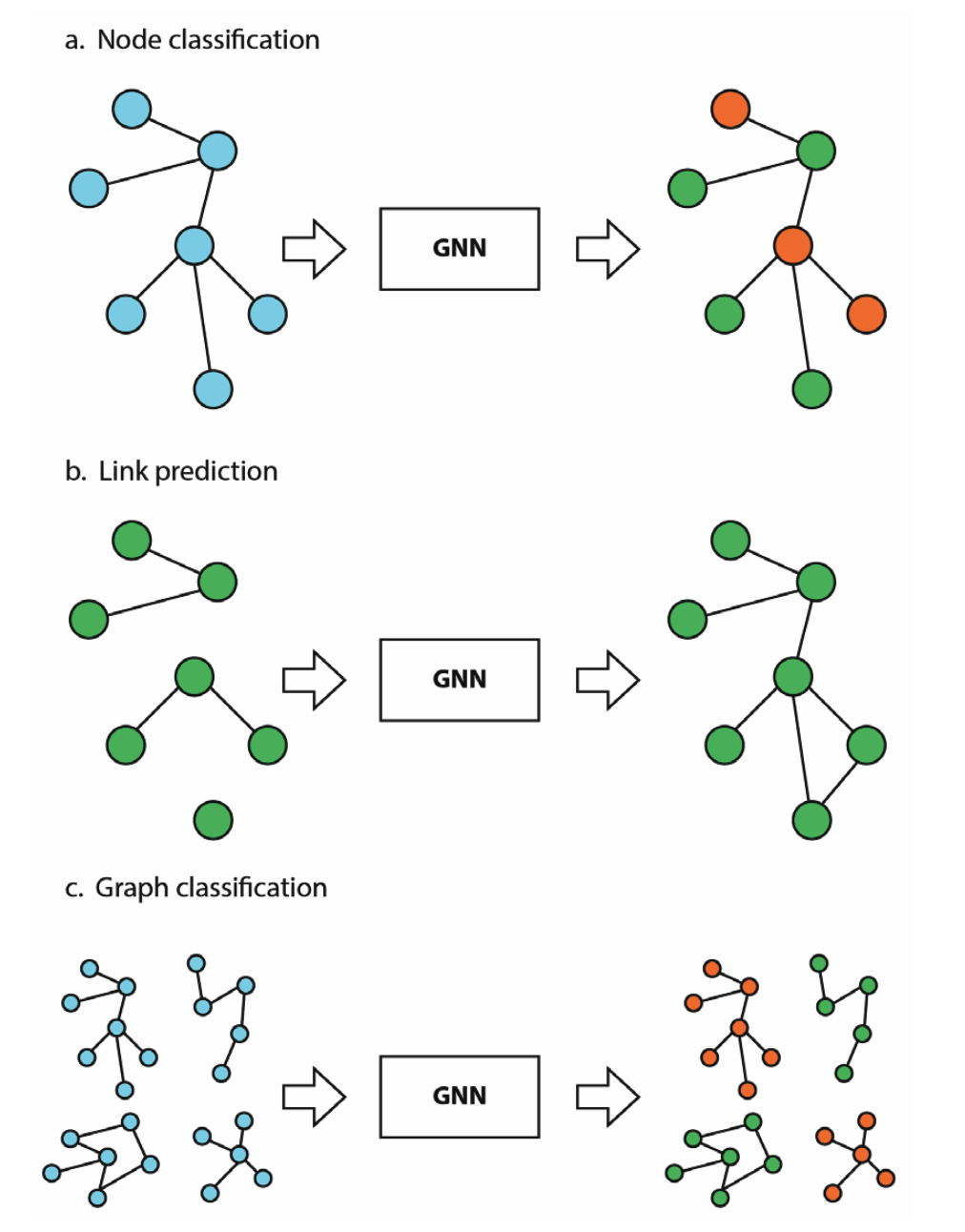 Figure 1: Graph learning tasks. Courtesy of [1].
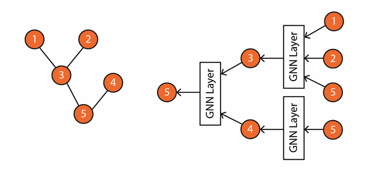 Figure 2: node 5’s representation is updated based on its neighbors. Courtesy of [1].
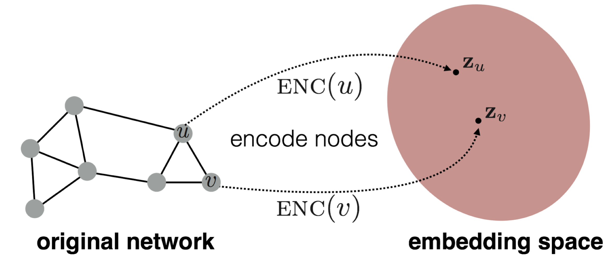 Figure 3: Encoder and decoder perspective. Courtesy of [2].
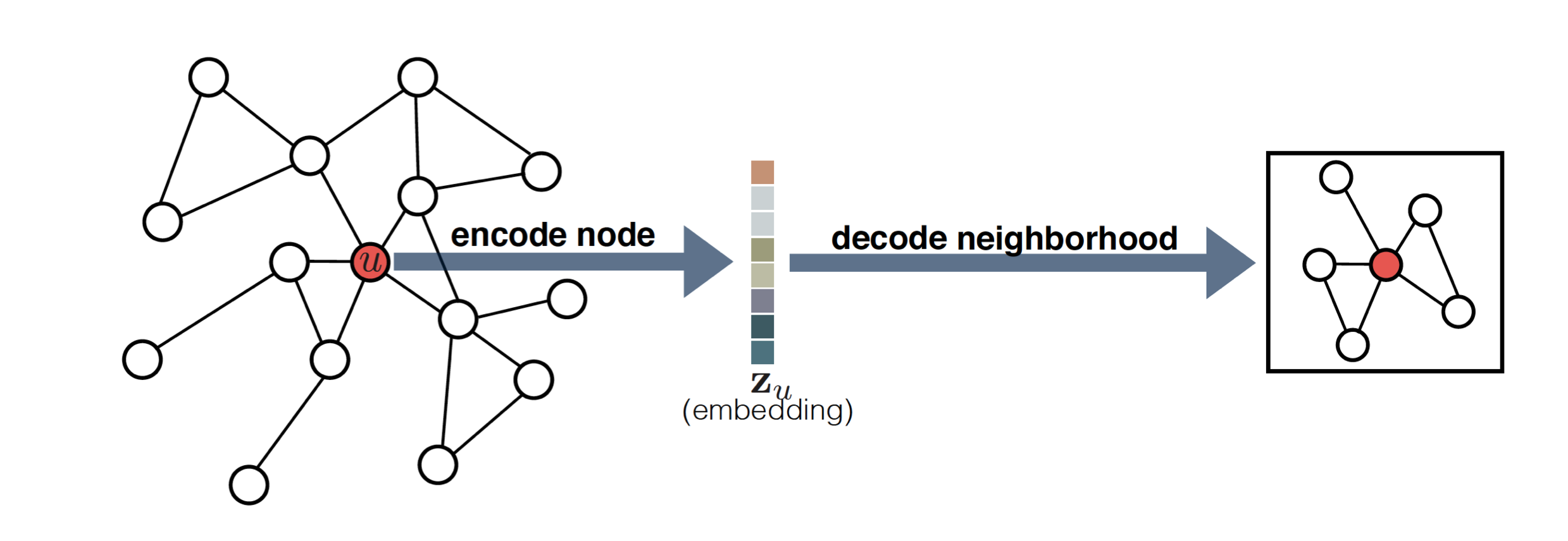 Figure 4: Encoder and decoder perspective. Courtesy of [2].
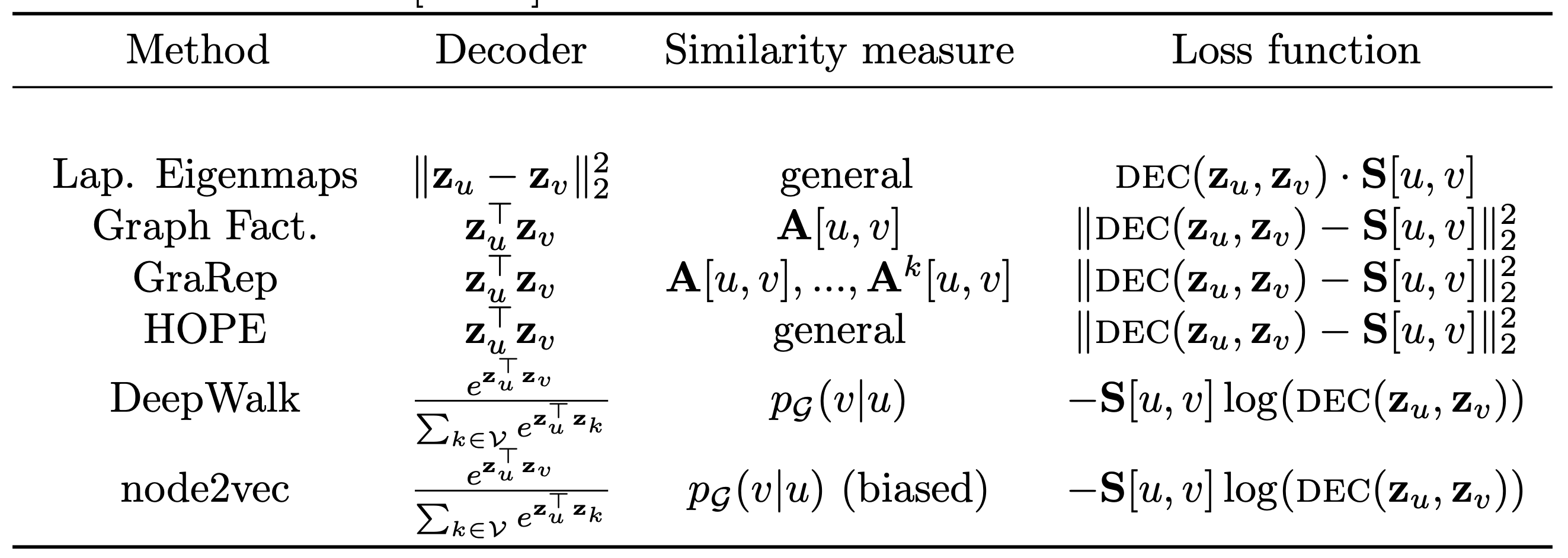 Table 1: Summary of some of the shallow embedding algorithms. Courtesy of [2].
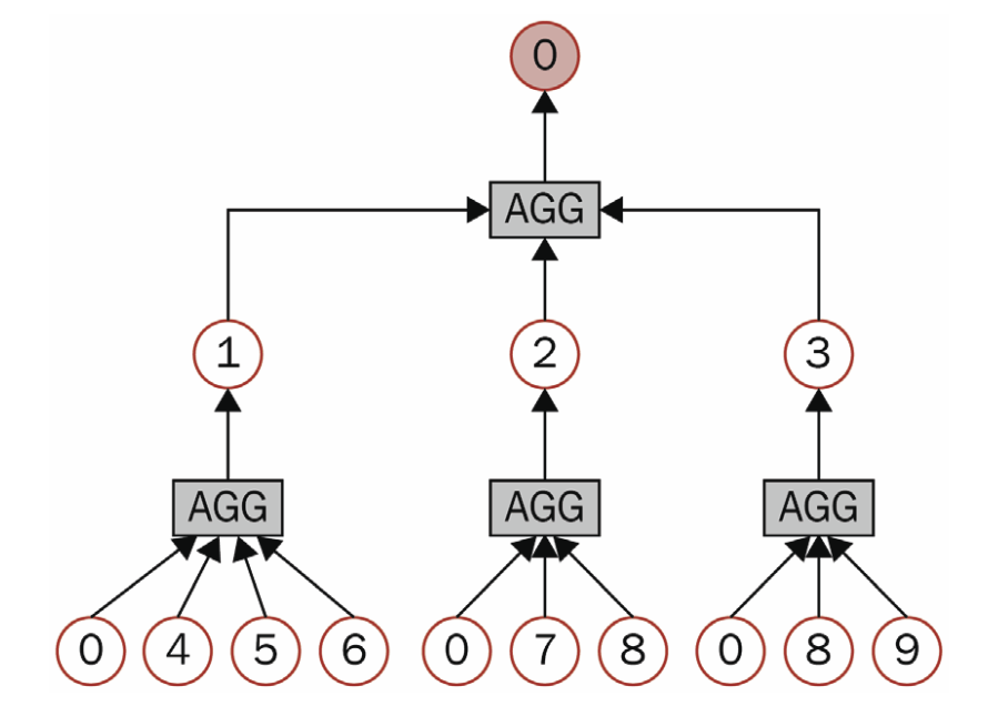 Figure 5: Computation graph for node 0. Courtesy of [1].
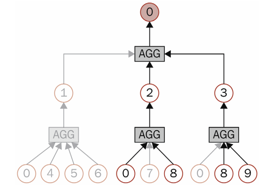 Figure 6: Computation graph with sampling for node 0. Courtesy of [1].
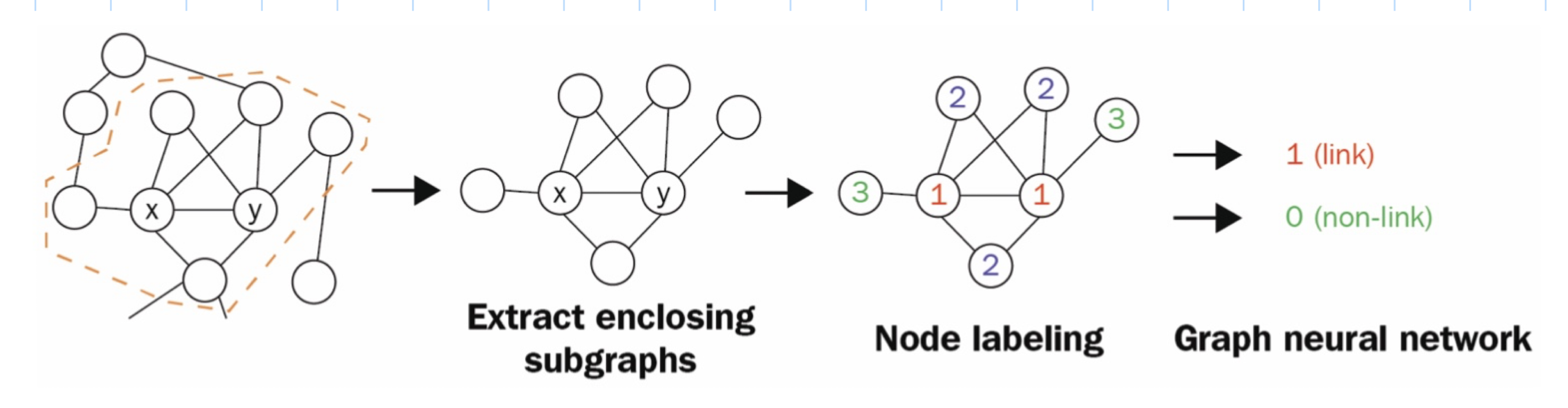 Figure 7: SEAL steps. Courtesy of [1].
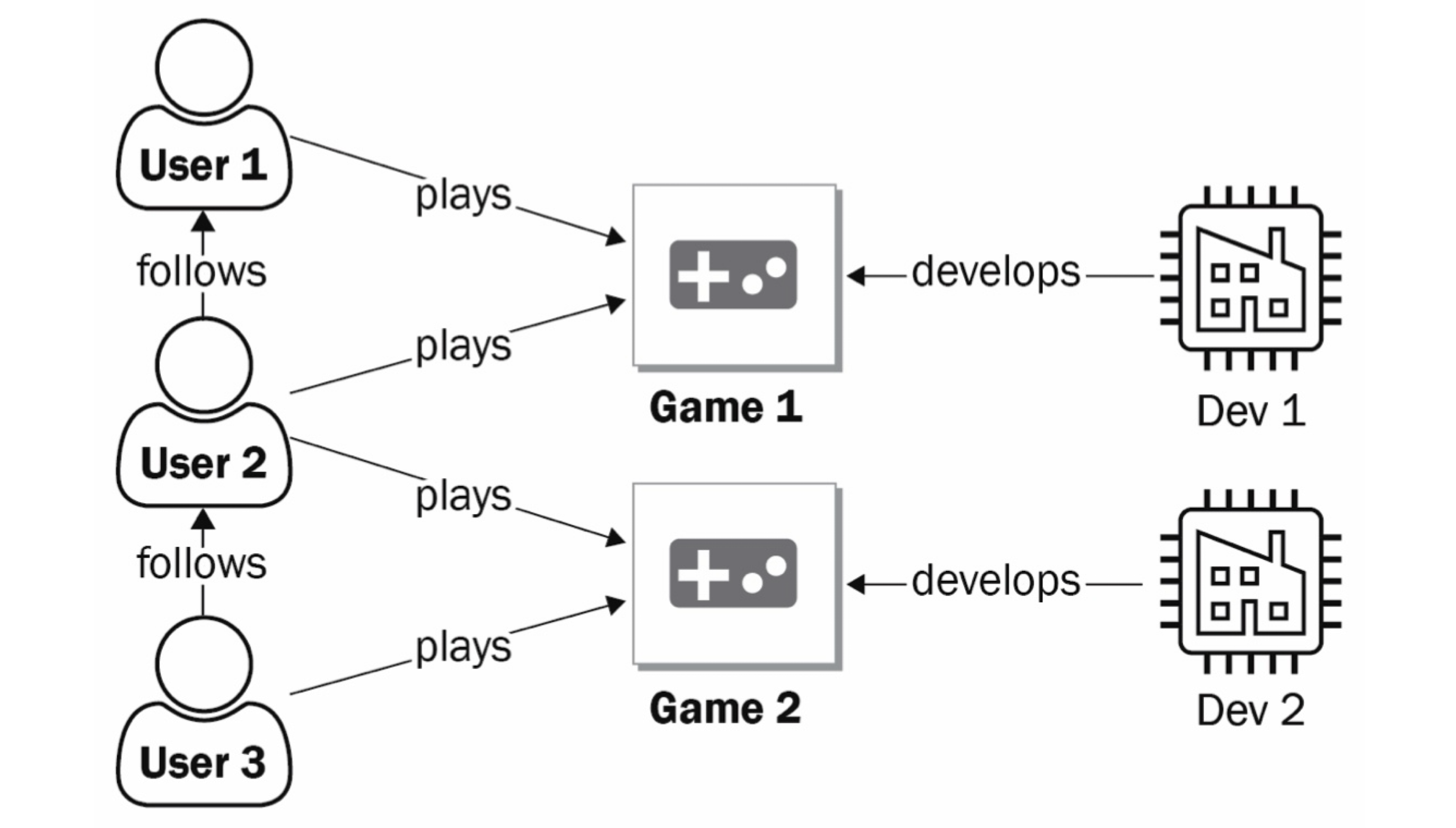 Figure 8: Heterogenous network. Courtesy of [1].