lecturenotes - Topic3 - Centrality in Networks

Degree of a node is a centrality metric. If a node has higher degree than the rest of the nodes of a network, it is more central in the network. However, degree is not the only centrality metric. There are other centrality metrics that can be used to measure the centrality of a node in a network. In this topic, we will learn about some of these centrality metrics.

Degree of node \(j\), \(d_j\) is calculated as:

\[ d_j = \sum_{i=1}^{n} A_{ij} \]

where \(A_{ij}\) is the element of the adjacency matrix of the network. In other words, degree of a node is the number of edges connected to that node. In a directed network, we can calculate the in-degree and out-degree of a node. In-degree is the number of edges pointing to a node and out-degree is the number of edges pointing from a node. In-degree and out-degree of a node is calculated as:

\[ d_{j(in)} = \sum_{i=1}^{n} A_{ij} \]

\[ d_{i(out)} = \sum_{j=1}^{n} A_{ij} \]

where \(A_{ij}\) is the element of the adjacency matrix of the network.

Closeness centrality of node \(j\), \(c_j\) is calculated as:

\[ c_j = \frac{1}{\sum_{i=1}^{n} d_{ij}} \]

where \(d_{ij}\) is the shortest path distance between node \(i\) and node \(j\). In other words, closeness centrality of a node is the inverse of the sum of the shortest path distances between that node and all other nodes in the network. Closeness centrality of a node is high if the node is close to all other nodes in the network. In other words, closeness centrality of a node is high if the node is reachable from all other nodes in the network with a short path.

Betweenness centrality of node \(j\) is calculated as:

\[ b_j = \sum_{s\neq t\neq j} \frac{\sigma_{st}(j)}{\sigma_{st}} \]

where \(\sigma_{st}\) is the number of shortest paths between node \(s\) and node \(t\) and \(\sigma_{st}(j)\) is the number of shortest paths between node \(s\) and node \(t\) that pass through node \(i\). In other words, betweenness centrality of a node is the fraction of shortest paths between all other nodes in the network that pass through that node. Betweenness centrality of a node is high if the node lies on many shortest paths between all other nodes in the network.

Eigenvector centrality (a nice video here) of a node is calculated as:

\[ x_j = \frac{1}{\lambda} \sum_{j=1}^{n} A_{ij} x_j \]

\[ Av = \lambda{v} \]

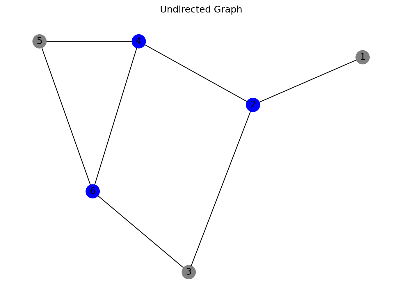
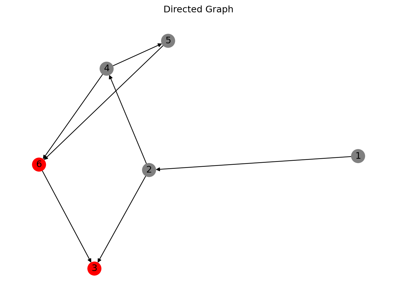
where \(A_{ij}\) is the element of the adjacency matrix of the network, \(x_i\) is the eigenvector centrality of node \(i\), \(x_j\) is the eigenvector centrality of node \(j\) and \(\lambda\) is the largest eigenvalue of the adjacency matrix. In other words, eigenvector centrality of a node is the sum of powers of all nodes connected to that node. Eigenvector centrality of a node is high if the node is connected to other nodes that have powers. Let’s get more into the eigenvector centrality computation. Observe node 4 in the first and node 3 in the second (i.e. directed) graph. Most influential? Similar to degree centrality with a feedback loop.

Find the largest eigenvalue of the adjacency matrix and the corresponding eigenvector. Then scale the vector so that it’s largest entry is 1. The eigenvector centrality of a node is the value of the corresponding eigenvector element. The eigenvector centrality of a node is high if the node is connected to other nodes that have high eigenvector centrality.

Code

import networkx as nx
import matplotlib.pyplot as plt

# Create the first undirected graph
G1 = nx.Graph()
edges1 = [(1, 2), (2, 3),  (2, 4), (6, 3), (4, 5), (4, 6), (5, 6) ]
G1.add_edges_from(edges1)

# Create the second directed graph
G2 = nx.DiGraph()
edges2 = [(1, 2), (2, 4), (2, 3), (4, 5), (4, 6), (5, 6), (6, 3)]
G2.add_edges_from(edges2)

# Create a dictionary to store node colors
node_colors1 = ['blue' if node in [2, 4, 6] else 'gray' for node in G1.nodes()]
node_colors2 = ['red' if node in [3, 6] else 'gray' for node in G2.nodes()]

# Draw the first graph
pos = nx.spring_layout(G1, seed=42)  # positions for all nodes
nx.draw(G1, pos, with_labels=True, node_color=node_colors1)
plt.title("Undirected Graph")
plt.show()

# Draw the second graph
pos = nx.spring_layout(G2, seed=42)  # positions for all nodes
nx.draw(G2, pos, with_labels=True, node_color=node_colors2)
plt.title("Directed Graph")
plt.show()

Code

# Calculate Eigenvector Centrality using NumPy
eigenvector_centrality1 = nx.eigenvector_centrality_numpy(G1, max_iter=500)
print(eigenvector_centrality1)

# Compute the eigenvector centrality of the nodes in the second graph
eigenvector_centrality2 = nx.eigenvector_centrality_numpy(G2, max_iter=500)
print(eigenvector_centrality2)

{1: 0.1604996091327092, 2: 0.40758614706919566, 3: 0.358307134172783, 4: 0.5162516483031148, 6: 0.5023289927498406, 5: 0.4010975248660488}
{1: 3.176266727862339e-14, 2: 1.5952942034480286e-11, 4: 7.97845977596604e-09, 3: 0.9999980009267192, 5: 3.990156207510809e-06, 6: 0.001999531606055718}

Code

print(list(G1.edges()))
print(G1.nodes())
A = nx.adjacency_matrix(G1).toarray()

[(1, 2), (2, 3), (2, 4), (3, 6), (4, 5), (4, 6), (6, 5)]
[1, 2, 3, 4, 6, 5]

Code

import numpy as np

def power_iteration(A, num_iterations=1000):
    n = A.shape[0]
    
    # Generate a random initial vector
    v = np.random.rand(n)
    
    for _ in range(num_iterations):
        Av = A.dot(v)
        v_new = Av / np.linalg.norm(Av)
        
        if np.allclose(v, v_new):
            break
        
        v = v_new
    
    eigenvalue = v.dot(Av)
    return eigenvalue, v

# Example usage
eigenvalue, eigenvector = power_iteration(A)

print("Dominant Eigenvalue:", eigenvalue)
print("Eigenvector:", eigenvector)

Dominant Eigenvalue: 2.539483736214395
Eigenvector: [0.16050046 0.40758433 0.35830863 0.51625318 0.50232761 0.40109746]

PageRank centrality (a nice video here) of a node is calculated as:

\[ x_i = \frac{1-d}{N} + d \sum_{j=1}^{n} \frac{A_{ij}}{d_{j}^{out}} x_j \]

where \(A_{ij}\) is the element of the adjacency matrix of the network, \(x_i\) is the PageRank centrality of node \(i\), \(x_j\) is the PageRank centrality of node \(j\), \(d\) is the damping factor and \(d_{j}^{out}\) is the out-degree of node \(j\). In other words, PageRank centrality of a node is the sum of the PageRank centrality of all nodes connected to that node. PageRank centrality of a node is high if the node is connected to other nodes that have high PageRank centrality.

In this topic, we will calculate the degree, in-degree, out-degree, closeness centrality, betweenness centrality, eigenvector centrality and PageRank centrality of nodes in a network.

Degree of a Node

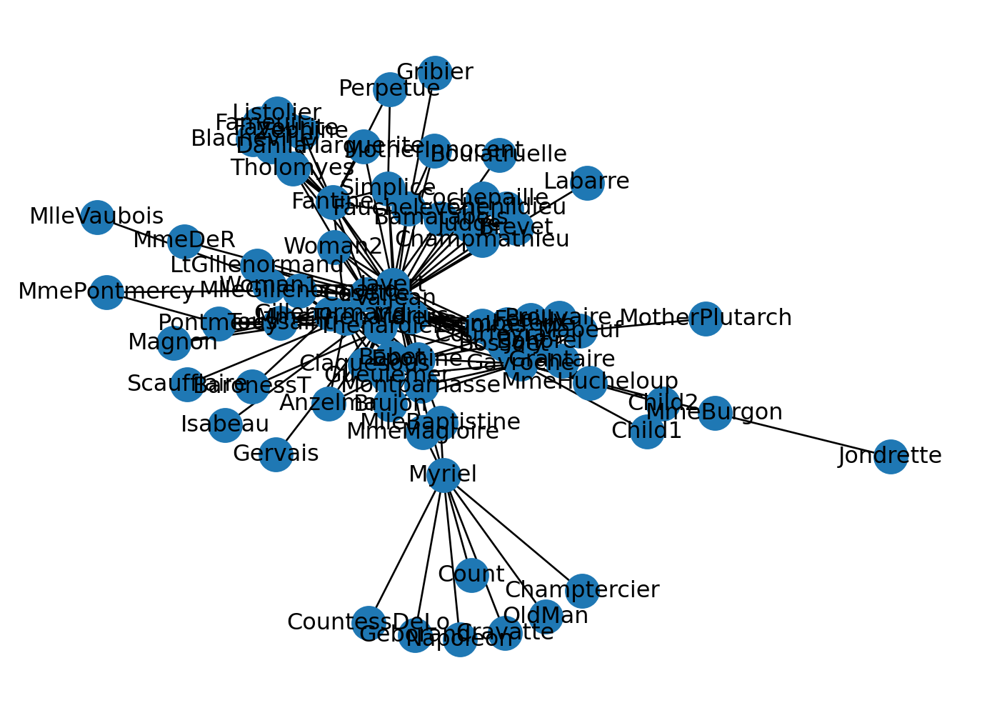
We will calculate the degree of a node in a network. We will use the network of the characters in the novel Les Miserables. The network is undirected. We will calculate the degree of each character in the network.

Code

import networkx as nx
import matplotlib.pyplot as plt

G = nx.les_miserables_graph()
nx.draw(G, with_labels=True)
plt.show()

Plot the most central character in the network.

Code

degree = nx.degree_centrality(G)
max_degree = max(degree.values())
max_degree_node = [k for k, v in degree.items() if v == max_degree]
print(max_degree_node)

['Valjean']

Color the most central character in the network.

Code

color_map = []
for node in G:
    if node == max_degree_node[0]:
        color_map.append('red')
    else:
        color_map.append('blue')
nx.draw(G, node_color=color_map, with_labels=True)
plt.show()

Closeness Centrality of a Node

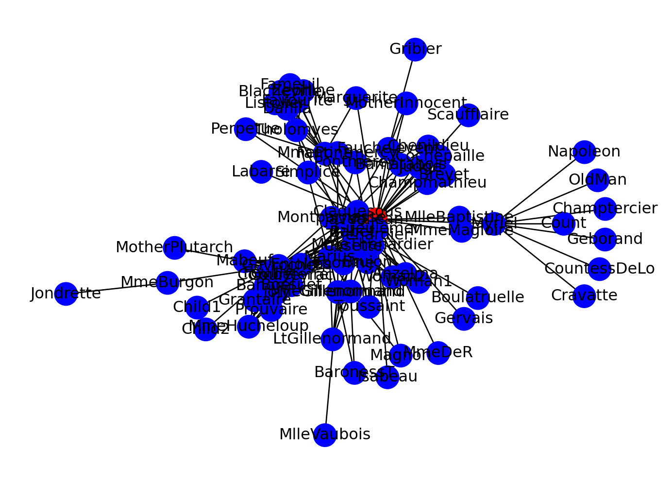
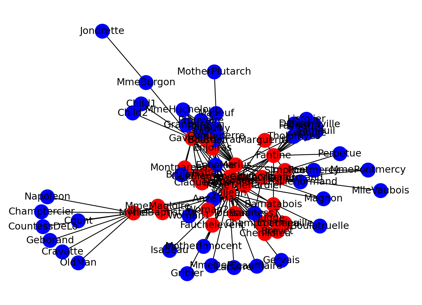
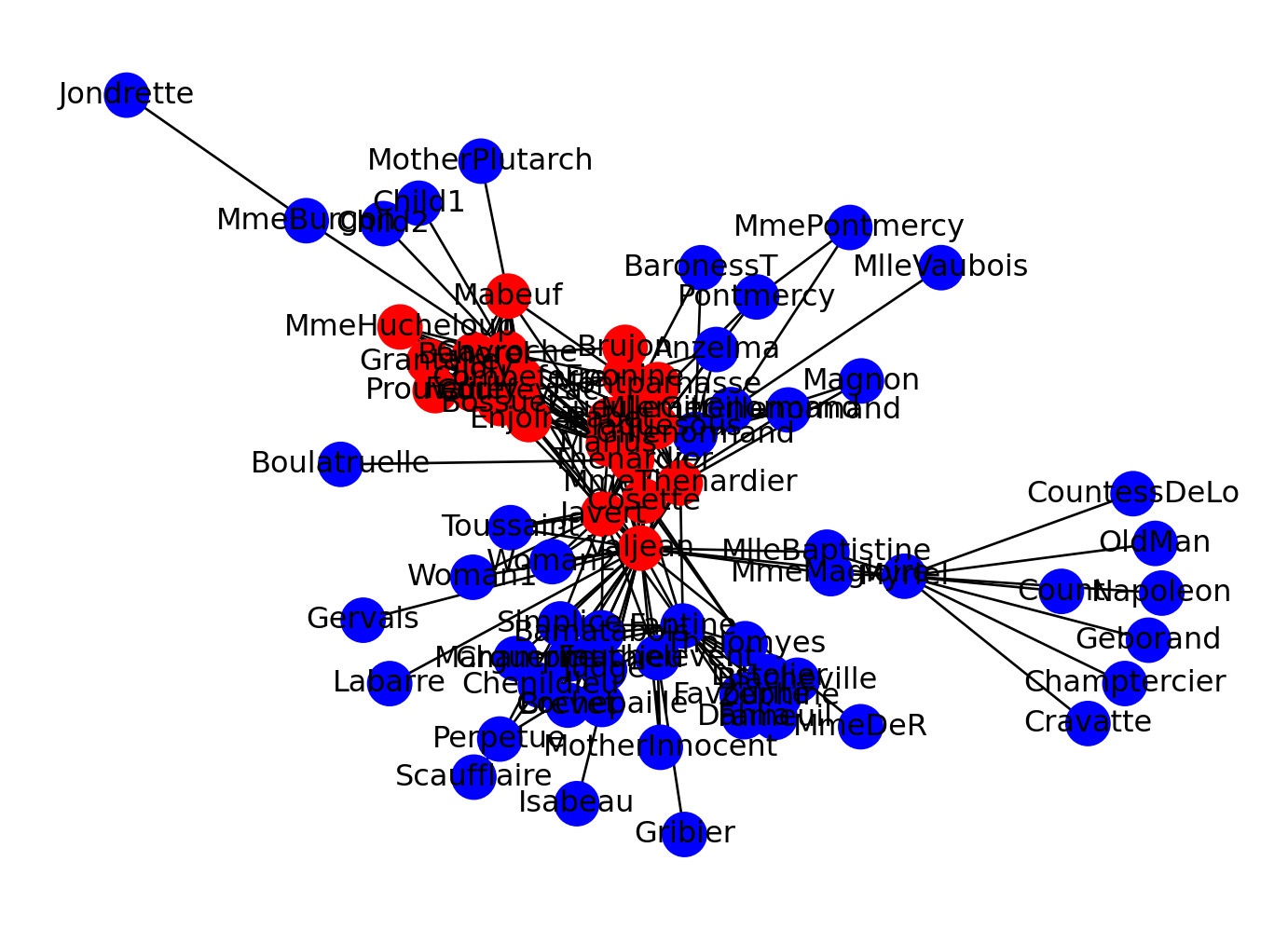
We will calculate the closeness centrality of a node in a network. We will use the network of the characters in the novel Les Miserables. The network is undirected. We will calculate the closeness centrality of each character in the network.

Code

import networkx as nx
import matplotlib.pyplot as plt

G = nx.les_miserables_graph()
#color the nodes according to their closeness centrality
closeness = nx.closeness_centrality(G)
color_map = []
for node in G:
    if closeness[node] > 0.4:
        color_map.append('red')
    else:
        color_map.append('blue')
nx.draw(G, node_color=color_map, with_labels=True)
plt.show()

If you want to use edge weights in the closeness centrality calculation, you can use the following code.

Code

import networkx as nx
import matplotlib.pyplot as plt

G = nx.les_miserables_graph()

# Calculate the inverse of weights as distance
for u, v, data in G.edges(data=True):
    if 'weight' in data:
        data['distance'] = 1 / data['weight']

# Color the nodes according to their closeness centrality
closeness = nx.closeness_centrality(G, distance='distance')
color_map = ['red' if closeness[node] > 1 else 'blue' for node in G.nodes()]

# Draw the graph
pos = nx.spring_layout(G)  # You can change the layout algorithm as needed
nx.draw(G, pos, node_color=color_map, with_labels=True)
plt.show()

Betweenness Centrality of a Node

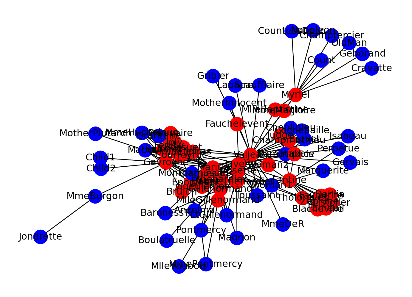
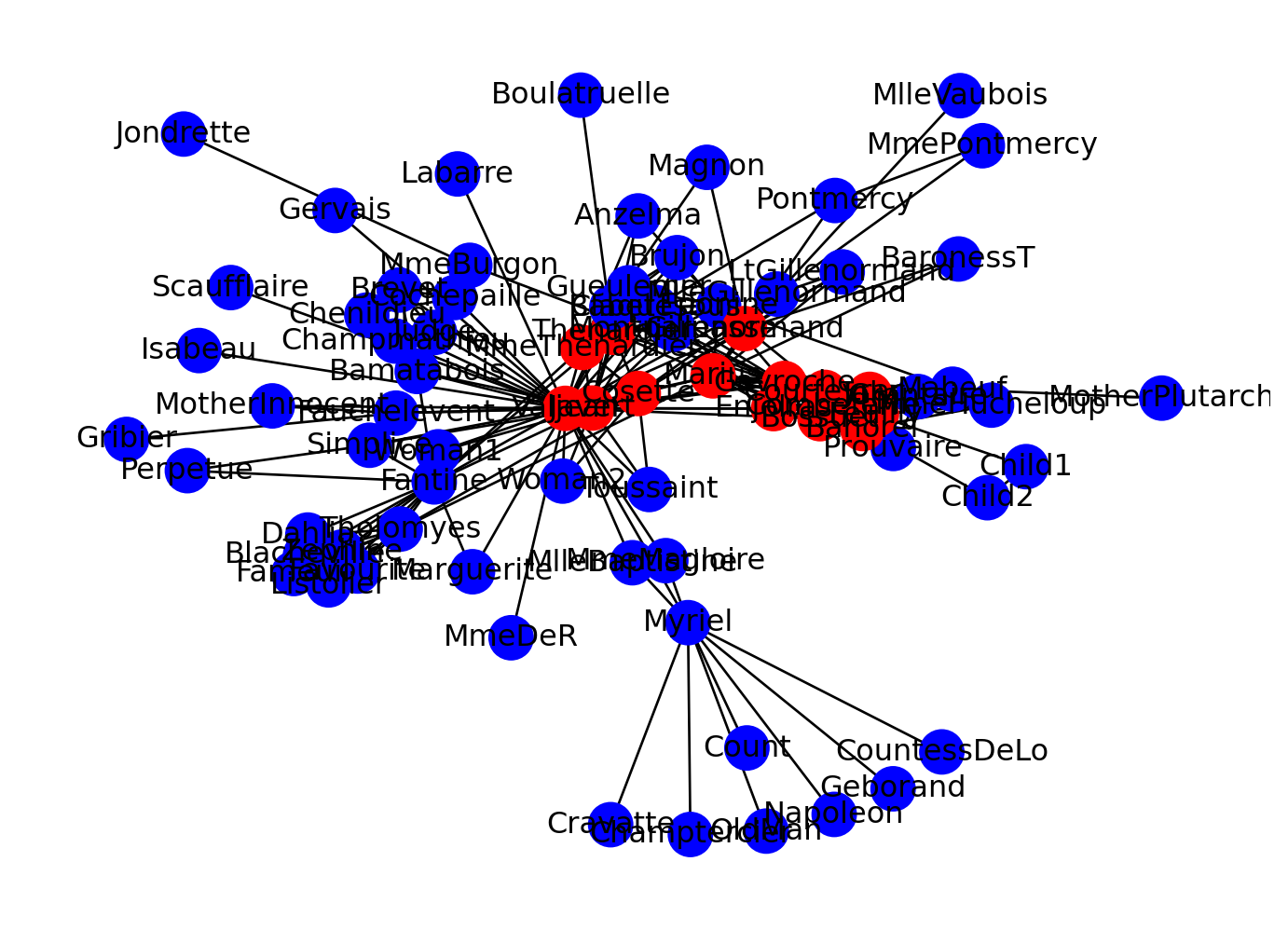
We will calculate the betweenness centrality of a node in a network. We will use the network of the characters in the novel Les Miserables. The network is undirected. We will calculate the betweenness centrality of each character in the network.

Code

import networkx as nx
import matplotlib.pyplot as plt

G = nx.les_miserables_graph()
#color the nodes according to their betweenness centrality
betweenness = nx.betweenness_centrality(G)
color_map = []
for node in G:
    if betweenness[node] > 0.05:
        color_map.append('red')
    else:
        color_map.append('blue')
nx.draw(G, node_color=color_map, with_labels=True)
plt.show()

We can use distance attribute to calculate the betweenness centrality of a node using edge weights. We will use the network of the characters in the novel Les Miserables. The network is undirected. We will calculate the betweenness centrality of each character in the network.

Code

import networkx as nx
import matplotlib.pyplot as plt
w_betweenness = nx.betweenness_centrality(G, weight='distance')
color_map = []
for node in G:
    if w_betweenness[node] > 0.05:
        color_map.append('red')
    else:
        color_map.append('blue')
nx.draw(G, node_color=color_map, with_labels=True)
plt.show()

Eigenvector Centrality of a Node

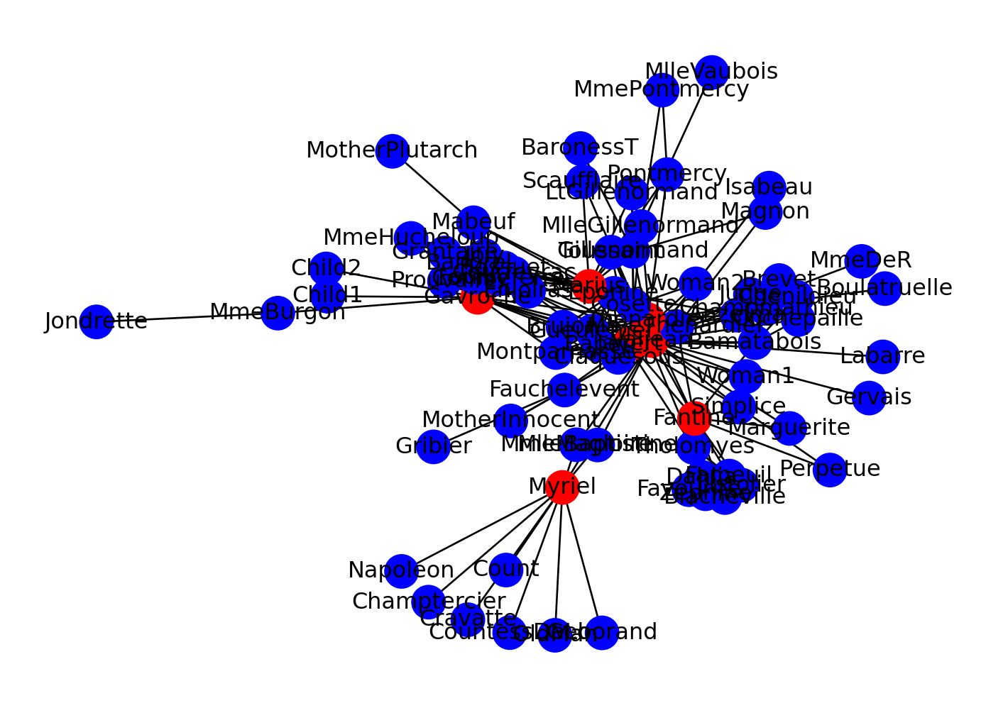
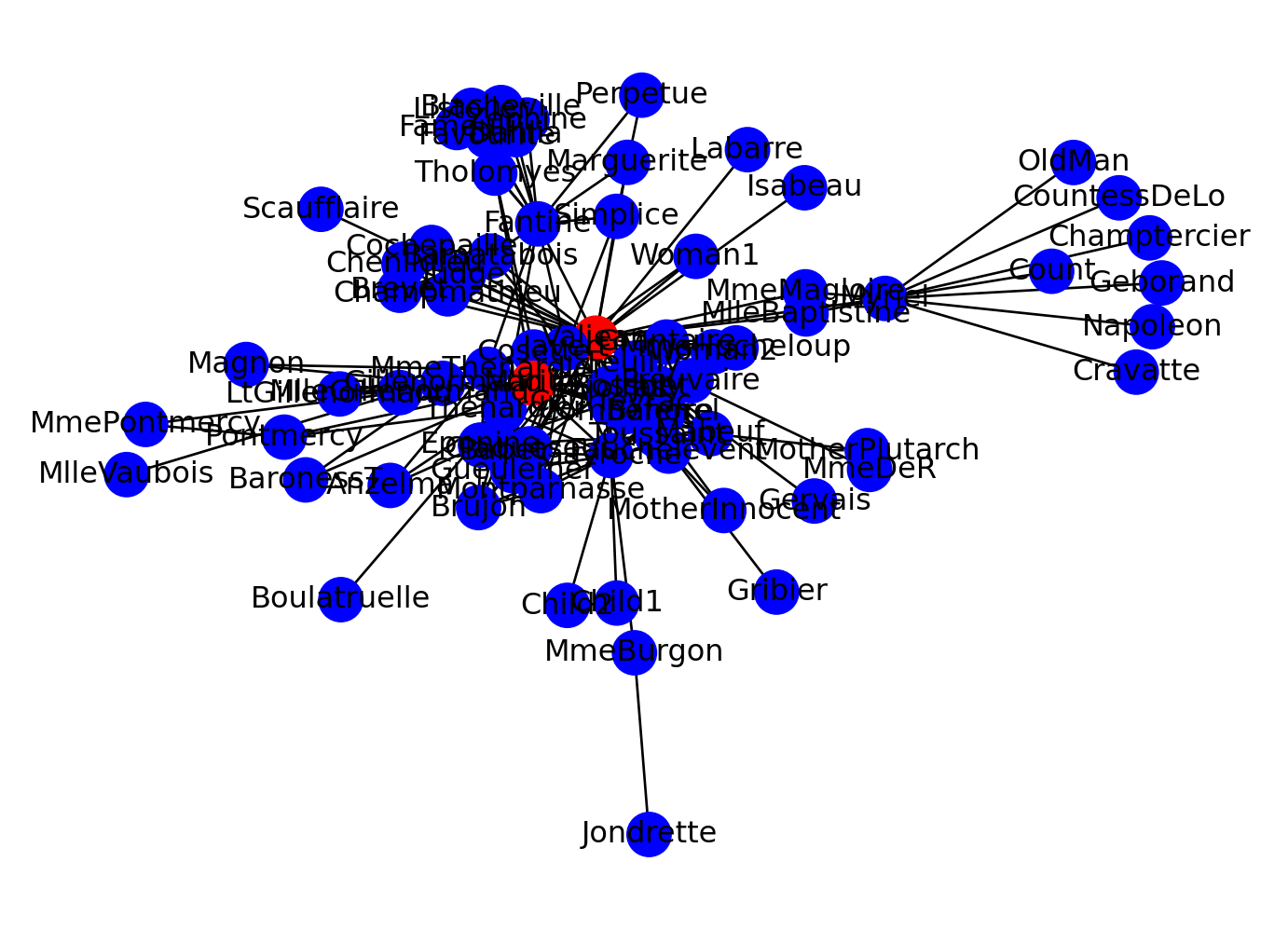
We will calculate the eigenvector centrality of a node in a network. We will use the network of the characters in the novel Les Miserables. The network is undirected. We will calculate the eigenvector centrality of each character in the network.

Code

import networkx as nx
import matplotlib.pyplot as plt

G = nx.les_miserables_graph()
#color the nodes according to their eigenvector centrality
eigenvector = nx.eigenvector_centrality(G)
color_map = []
for node in G:
    if eigenvector[node] > 0.1:
        color_map.append('red')
    else:
        color_map.append('blue')
nx.draw(G, node_color=color_map, with_labels=True)
plt.show()

We can use edge weights to calculate weighted eigenvector centrality.

Code

import networkx as nx
import matplotlib.pyplot as plt

G = nx.les_miserables_graph()
#color the nodes according to their eigenvector centrality
w_eigenvector = nx.eigenvector_centrality(G, weight='weight')
color_map = []
for node in G:
    if w_eigenvector[node] > 0.1:
        color_map.append('red')
    else:
        color_map.append('blue')
nx.draw(G, node_color=color_map, with_labels=True)
plt.show()

PageRank Centrality of a Node

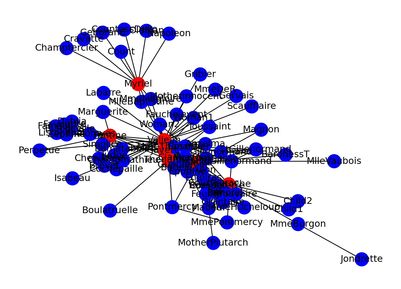
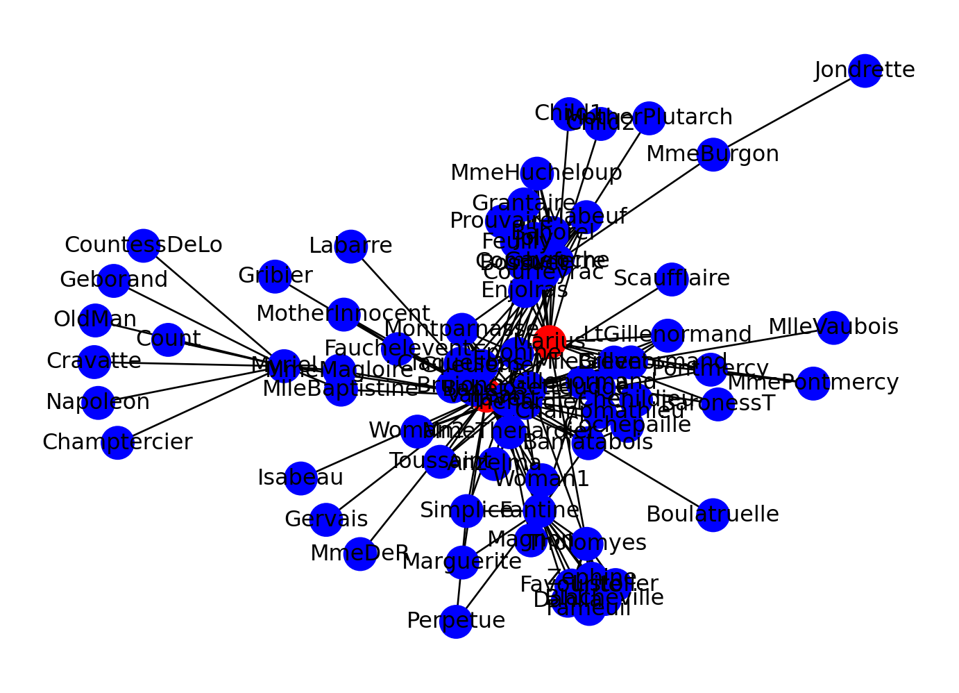
We will calculate the PageRank centrality of a node in a network. We will use the network of the characters in the novel Les Miserables. The network is undirected. We will calculate the PageRank centrality of each character in the network.

Code

import networkx as nx
import matplotlib.pyplot as plt

G = nx.les_miserables_graph()
#color the nodes according to their PageRank centrality
pagerank = nx.pagerank(G)
color_map = []
for node in G:
    if pagerank[node] > 0.05:
        color_map.append('red')
    else:
        color_map.append('blue')
nx.draw(G, node_color=color_map, with_labels=True)
plt.show()

We can use edge weights to calculate weighted PageRank centrality.

Code

import networkx as nx
import matplotlib.pyplot as plt

G = nx.les_miserables_graph()
#color the nodes according to their PageRank centrality
w_pagerank = nx.pagerank(G, weight='weight')
color_map = []
for node in G:
    if w_pagerank[node] > 0.05:
        color_map.append('red')
    else:
        color_map.append('blue')
nx.draw(G, node_color=color_map, with_labels=True)
plt.show()

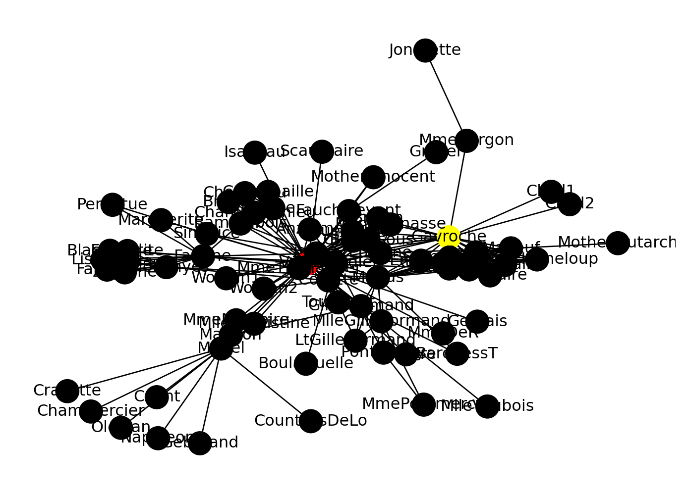
Plot the most central characters in different colors based on degree, closeness centrality, betweenness centrality, eigenvector centrality and PageRank centrality.

Code

import networkx as nx
import matplotlib.pyplot as plt

G = nx.les_miserables_graph()
#color the nodes according to their degree
degree = nx.degree_centrality(G)
max_degree = max(degree.values())
max_degree_node = [k for k, v in degree.items() if v == max_degree]
#color the nodes according to their closeness centrality
closeness = nx.closeness_centrality(G)
max_closeness = max(closeness.values())
max_closeness_node = [k for k, v in closeness.items() if v == max_closeness]
#color the nodes according to their betweenness centrality
betweenness = nx.betweenness_centrality(G)
max_betweenness = max(betweenness.values())
max_betweenness_node = [k for k, v in betweenness.items() if v == max_betweenness]
#color the nodes according to their eigenvector centrality
eigenvector = nx.eigenvector_centrality(G)
max_eigenvector = max(eigenvector.values())
max_eigenvector_node = [k for k, v in eigenvector.items() if v == max_eigenvector]
#color the nodes according to their PageRank centrality
pagerank = nx.pagerank(G)
max_pagerank = max(pagerank.values())
max_pagerank_node = [k for k, v in pagerank.items() if v == max_pagerank]
color_map = []
for node in G:
    if node in max_degree_node:
        color_map.append('red')
    elif node in max_closeness_node:
        color_map.append('blue')
    elif node in max_betweenness_node:
        color_map.append('green')
    elif node in max_eigenvector_node:
        color_map.append('yellow')
    elif node in max_pagerank_node:
        color_map.append('purple')
    else:
        color_map.append('black')
nx.draw(G, node_color=color_map, with_labels=True)
plt.show()

If a node has maximum cenrality in more than one centrality measure, it will be colored according to the first centrality measure in the above code.

Which nodes have maximum centrality in more than one centrality measure?

Code

import networkx as nx
import matplotlib.pyplot as plt

G = nx.les_miserables_graph()
#which nodes have maximum centrality in more than one centrality measure?
degree = nx.degree_centrality(G)
max_degree = max(degree.values())
max_degree_node = [k for k, v in degree.items() if v == max_degree]
closeness = nx.closeness_centrality(G)
max_closeness = max(closeness.values())
max_closeness_node = [k for k, v in closeness.items() if v == max_closeness]
betweenness = nx.betweenness_centrality(G)
max_betweenness = max(betweenness.values())
max_betweenness_node = [k for k, v in betweenness.items() if v == max_betweenness]
eigenvector = nx.eigenvector_centrality(G)
max_eigenvector = max(eigenvector.values())
max_eigenvector_node = [k for k, v in eigenvector.items() if v == max_eigenvector]
pagerank = nx.pagerank(G)
max_pagerank = max(pagerank.values())
max_pagerank_node = [k for k, v in pagerank.items() if v == max_pagerank]
print(max_degree_node)
print(max_closeness_node)
print(max_betweenness_node)
print(max_eigenvector_node)
print(max_pagerank_node)

['Valjean']
['Valjean']
['Valjean']
['Gavroche']
['Valjean']

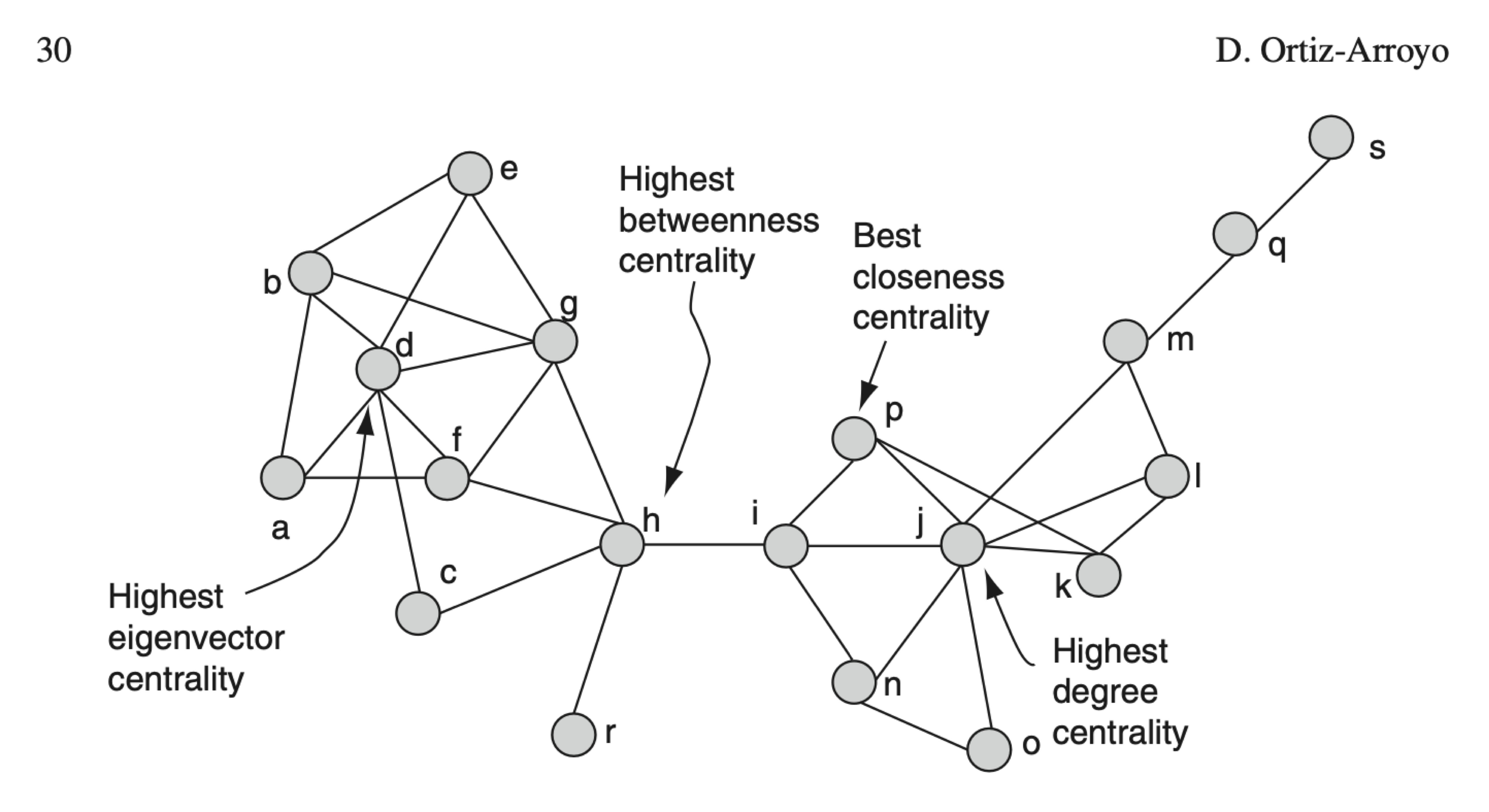
Figure 1 illustrates how each centrality metric can idenrify different central nodes in a network.

Alt Text — Figure 1: central nodes based on different centrality metrics.

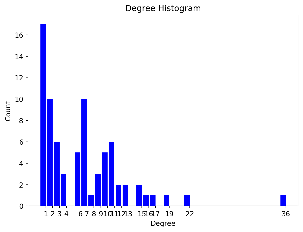
Degree Distribution

We will plot the degree distribution of a network. We will use the network of the characters in the novel Les Miserables. The network is undirected.

Code

import networkx as nx
import matplotlib.pyplot as plt
import collections

G = nx.les_miserables_graph()
degree_sequence = sorted([d for n, d in G.degree()], reverse=True)
degreeCount = collections.Counter(degree_sequence)
deg, cnt = zip(*degreeCount.items())
fig, ax = plt.subplots()
plt.bar(deg, cnt, width=0.80, color='b')
plt.title("Degree Histogram")
plt.ylabel("Count")
plt.xlabel("Degree")
ax.set_xticks([d + 0.4 for d in deg])
ax.set_xticklabels(deg)
plt.show()

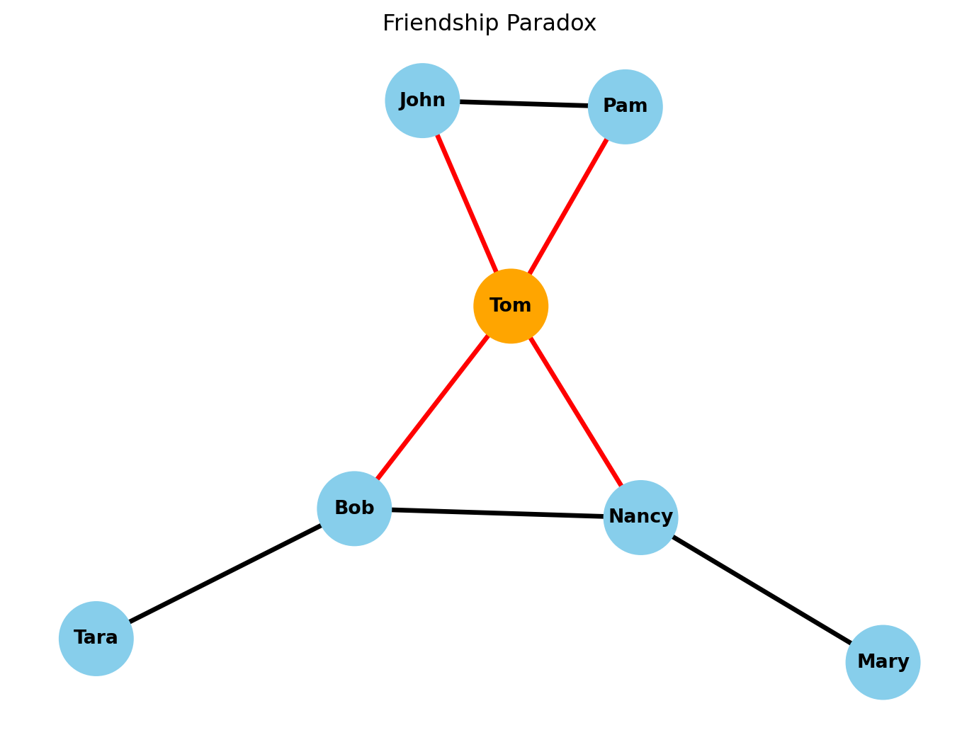
Friendship Paradox

We will show that the average degree of the neighbors of a node is higher than the average degree of the nodes in the network. We will use the network of people illustrated below (Courtesy of Reference 1 Section 8).

Code

import networkx as nx
import matplotlib.pyplot as plt

# Create an empty graph
G = nx.Graph()

# Define the nodes
nodes = ["Mary", "Nancy", "Tom", "Tara", "Bob", "Pam", "John"]

# Add nodes to the graph
G.add_nodes_from(nodes)

# Define the edges
edges = [("Mary", "Nancy"),
         ("Nancy", "Tom"),
         ("Nancy", "Bob"),
         ("Bob", "Tara"),
         ("Tom", "John"),
         ("Tom", "Pam"),
         ("Tom", "Bob"),
         ("John", "Pam")]

# Add edges to the graph
G.add_edges_from(edges)

# Draw the graph
pos = nx.spring_layout(G)  # Position the nodes using a spring layout

# Define node colors
node_colors = ["skyblue" if node != "Tom" else "orange" for node in G.nodes()]

# Define edge colors
edge_colors = ["red" if "Tom" in edge else "black" for edge in G.edges()]

nx.draw(G, pos, with_labels=True, node_size=1500, node_color=node_colors, font_size=10, font_color="black", font_weight="bold", edge_color=edge_colors, width=2.5)
plt.title("Friendship Paradox")
plt.show()

# Calculate the average degree of the nodes in the network
avg_degree = sum([d for n, d in G.degree()]) / len(G.nodes())
print(f"Average degree of the nodes in the network: {avg_degree:.2f}") 
# Calculate the average degree of the neighbors in the network
avg_neighbor_degree = nx.average_neighbor_degree(G)
avg_neighbor_degree = sum([d for n, d in avg_neighbor_degree.items()]) / len(avg_neighbor_degree)
print(f"Average degree of the neighbors in the network: {avg_neighbor_degree:.2f}")

Average degree of the nodes in the network: 2.29
Average degree of the neighbors in the network: 2.83

The probability of the highest degree node to be reached is \(1/7\). The probability of selecting a random friend of a random individual is \[1/7 \times (1/3+1/3+1/2+1/2) = 5/21\]

Our friends have more friends than we have on average!

references

1: Network science textbook