It’s time to get back to basics

John Major

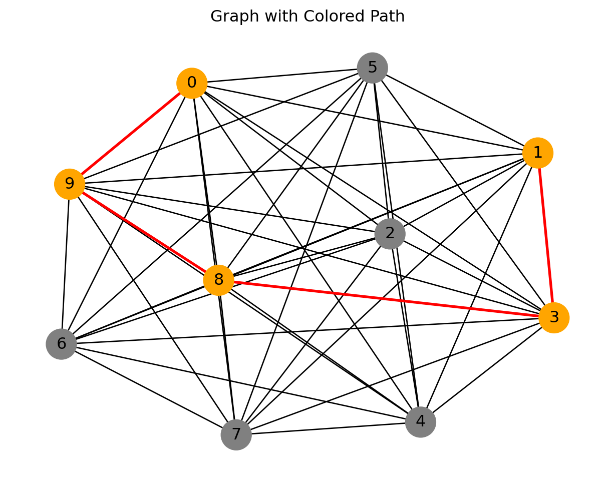
A path is a walk with distinct nodes (what’s a walk?)

We can define a walk as:

\[W = (v_0, e_1, v_1, e_2, v_2, ..., e_n, v_n)\]

where \(v_i\) is a node and \(e_i\) is an edge.

Code

import networkx as nx
import numpy as np
import matplotlib.pyplot as plt

def generate_path(G, length):
    nodes = list(G.nodes())
    current_node = nodes[0]
    path = [current_node]
    for _ in range(1, length):
        next_node = np.random.choice(nodes)
        while next_node in path:
            next_node = np.random.choice(nodes)
        path.append(next_node)
    return path

G = nx.Graph()
G.add_nodes_from(range(10))
for i in range(10):
    for j in range(i + 1, 10):
        G.add_edge(i, j)
#nx.draw_networkx(G)
path = generate_path(G, 5)
print(path)

# Create a list of colors for the nodes in the path
node_colors = ['orange' if node in path else 'gray' for node in G.nodes()]

# Draw the graph with colored nodes
plt.figure(figsize=(8, 6))
pos = nx.spring_layout(G)  # Positions for all nodes
nx.draw_networkx(G, pos, node_color=node_colors, node_size=500, font_size=12, with_labels=True)

# Draw the path edges separately to highlight them
path_edges = list(zip(path[:-1], path[1:]))
nx.draw_networkx_edges(G, pos, edgelist=path_edges, edge_color='red', width=2)

# Set plot title and show the graph
plt.title('Graph with Colored Path')
plt.axis('off')
plt.show()

[0, 9, 8, 3, 1]

Let’s generate a random path on a graph that is not complete.

Code

import networkx as nx
import random

# Create a graph (replace this with your actual graph creation)
G = nx.complete_bipartite_graph(3, 5)
# Add nodes and edges to the graph here...

# Function to generate a random path of a given length
def generate_random_path(graph, path_length):
    if path_length < 1:
        raise ValueError("Path length must be at least 1")
    if path_length > len(graph.nodes) - 1:
        raise ValueError("Path length exceeds the number of nodes - 1")

    # Select a random starting node
    start_node = random.choice(list(graph.nodes))

    # Initialize the path with the starting node
    path = [start_node]

    for _ in range(path_length):
        # Get neighbors of the current node
        neighbors = list(graph.neighbors(path[-1]))

        # Remove nodes that are already in the path to prevent loops
        valid_neighbors = [n for n in neighbors if n not in path]

        if not valid_neighbors:
            # If there are no valid neighbors, break the loop
            break

        # Select a random neighbor to extend the path
        next_node = random.choice(valid_neighbors)

        # Add the next node to the path
        path.append(next_node)

    return path

# Specify the desired path length
path_length = 5

try:
    # Generate a random path
    random_path = generate_random_path(G, path_length)
    print("Random Path:", random_path)
except ValueError as e:
    print(e)

Random Path: [3, 0, 5, 2, 7, 1]

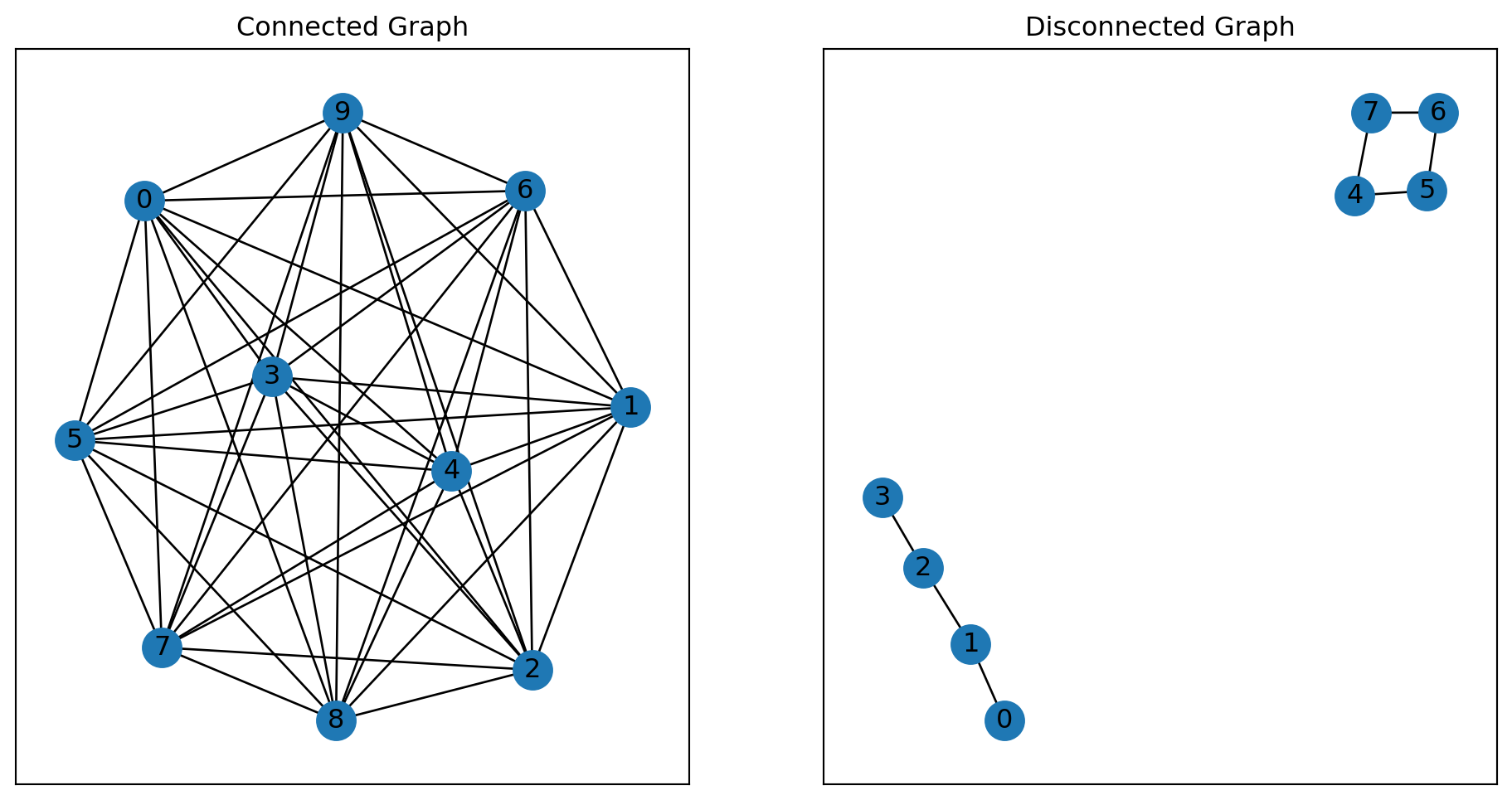
Connected Graph

A graph is connected if there is a path between every pair of vertices. In a connected graph, there are no unreachable vertices. A graph that is not connected is disconnected. A graph is disconnected if there exist two nodes \(u\) and \(v\) in \(G\) such that there is no path from \(u\) to \(v\).

Note that in directed graphs, we define strong connectivity and weak connectivity. A directed graph is strongly connected if there is a path between all pairs of vertices. A directed graph is weakly connected if there is a path between all pairs of vertices when the direction of the edges is ignored.

Graph laplacian of a connected graph has only one zero eigenvalue.

Code

import numpy as np
import networkx as nx

# Create a graph (replace this with your actual graph creation)
G = nx.complete_bipartite_graph(3, 5)

# Calculate the Laplacian matrix
laplacian_matrix = nx.laplacian_matrix(G).toarray()

# Find the eigenvalues of the Laplacian matrix
eigenvalues = np.linalg.eigvals(laplacian_matrix)
print(eigenvalues)

# Check if there is exactly one eigenvalue equal to zero
num_zero_eigenvalues = np.count_nonzero(np.isclose(eigenvalues, 0))

if num_zero_eigenvalues == 1:
    print("The graph is connected.")
else:
    print("The graph is not connected.")

[0. 5. 8. 5. 3. 3. 3. 3.]
The graph is connected.

Code

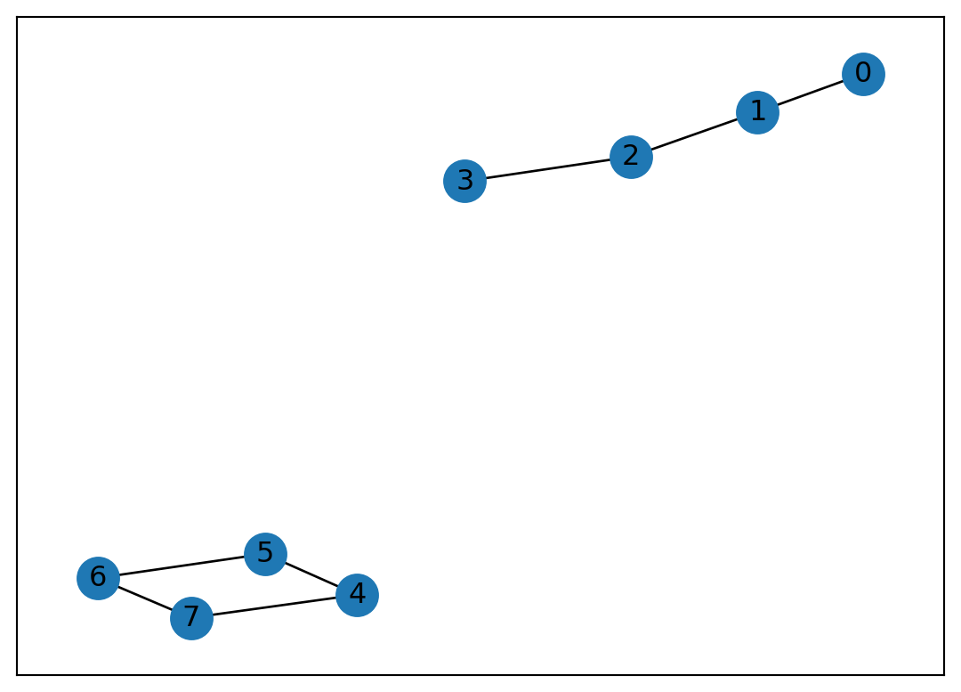
import networkx as nx
import matplotlib.pyplot as plt

# Generate a connected graph
connected_graph = nx.complete_graph(10)

# Generate a disconnected graph with two components
disconnected_graph = nx.Graph()
disconnected_graph.add_edges_from([(0, 1),(1,2), (2, 3), (4, 5),(4,7),(5,6),(6, 7)])


# Create a figure and axes
fig, axes = plt.subplots(1, 2, figsize=(12, 6))

# Draw the connected graph
pos_connected = nx.spring_layout(connected_graph)
nx.draw_networkx(connected_graph, pos=pos_connected, ax=axes[0], with_labels=True)
axes[0].set_title('Connected Graph')

# Draw the disconnected graph
pos_disconnected = nx.spring_layout(disconnected_graph)
nx.draw_networkx(disconnected_graph, pos=pos_disconnected, ax=axes[1], with_labels=True)
axes[1].set_title('Disconnected Graph')

# Hide the axis ticks and labels
for ax in axes:
    ax.set_xticks([])
    ax.set_yticks([])

# Adjust the spacing between subplots
plt.subplots_adjust(wspace=0.2)

# Show the plot
plt.show()

nx.is_connected(connected_graph)
nx.is_connected(disconnected_graph)

print(nx.number_connected_components(disconnected_graph))
print(list(nx.connected_components(disconnected_graph)))

nx.node_connected_component(disconnected_graph, 5)

2
[{0, 1, 2, 3}, {4, 5, 6, 7}]

{4, 5, 6, 7}

How many edges or nodes would need to be removed to increase the number of components of a network? Remember, a connected network is a single component and depending on the disconnectivity a network might have several components. Giant components including more nodes are usually matter of interest.

Code

print("Number of edge removals(cut) needed to disconnect network: {}".format(nx.edge_connectivity(connected_graph)))
print("Number of cuts needed to cut connection between node 1 and 2: {}".format(nx.edge_connectivity(disconnected_graph, 1 , 2)))

Number of edge removals(cut) needed to disconnect network: 9
Number of cuts needed to cut connection between node 1 and 2: 1

what are these edges?

Code

print(nx.minimum_edge_cut(connected_graph))
print(nx.minimum_edge_cut(disconnected_graph, 1, 2))

{(0, 1), (0, 7), (0, 4), (0, 3), (0, 9), (0, 6), (0, 2), (0, 5), (0, 8)}
{(1, 2)}

see how connected_graph becomes disconnected once we remove these edges

Code

import networkx as nx
removeE = nx.minimum_edge_cut(connected_graph)
updated_graph = connected_graph.copy()
updated_graph.remove_edges_from(removeE)
print(nx.number_connected_components(updated_graph))

similarly, there are cut vertices or nodes that once removed, the network becomes disconnected.

Code

print("Number of node removals(cut) needed to disconnect network: {}".format(nx.node_connectivity(connected_graph)))
print("Number of cuts needed to cut connection between node 1 and 2: {}".format(nx.node_connectivity(disconnected_graph, 1 , 2)))

Number of node removals(cut) needed to disconnect network: 9
Number of cuts needed to cut connection between node 1 and 2: 1

which nodes are these?

Code

print(nx.minimum_node_cut(connected_graph))
print(nx.minimum_node_cut(disconnected_graph, 1, 3))

{1, 2, 3, 4, 5, 6, 7, 8, 9}
{2}

see how connected_graph becomes disconnected once we remove these nodes

Code

import networkx as nx
removeN = nx.minimum_node_cut(connected_graph)
updated_graph = connected_graph.copy()
updated_graph.remove_nodes_from(removeN)
print(nx.number_connected_components(updated_graph))

Shortest paths are used in many applications such as routing, network analysis, and social network analysis.

Code

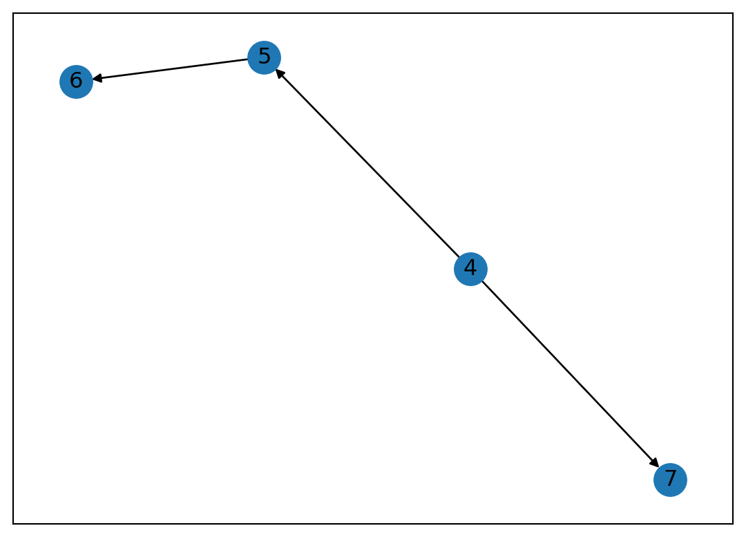
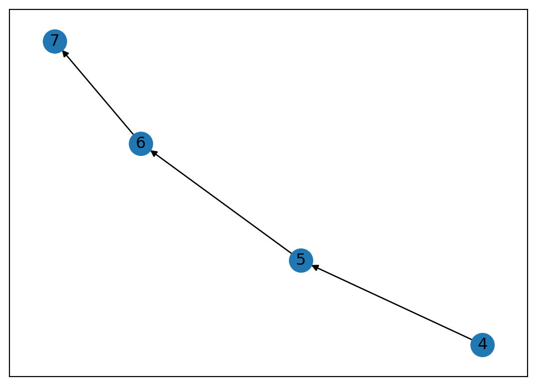
print("Length of the shortest path between nodes 4 and 6:")
print(nx.shortest_path_length(disconnected_graph, 4, 6))
print("Associated path:")
print(nx.shortest_path(disconnected_graph, 4, 6))

Length of the shortest path between nodes 4 and 6:
2
Associated path:
[4, 5, 6]

Shortest paths from a node to all other nodes in the network

Code

nx.shortest_path_length(disconnected_graph, 4)
nx.draw_networkx(disconnected_graph)

Breadth first search (BFS) is an algorithm for traversing or searching tree or graph data structures. It starts at the tree root (or some arbitrary node of a graph, sometimes referred to as a ‘search key’[1]) and explores the neighbor nodes first, before moving to the next level neighbors.

Code

nx.bfs_tree(disconnected_graph, 4)
nx.draw_networkx(nx.bfs_tree(disconnected_graph, 4))

We can use BFS to conclude if a graph is connected or not. If BFS visits all nodes, then the graph is connected. If BFS doesn’t visit all nodes, then the graph is disconnected.

Code

import networkx as nx
import random

# Create a random graph with a given number of nodes and edges
def generate_random_network(num_nodes, num_edges):
    G = nx.Graph()
    nodes = range(num_nodes)
    G.add_nodes_from(nodes)
    
    if num_edges > num_nodes * (num_nodes - 1) // 2:
        raise ValueError("Too many edges for the given number of nodes")
    
    edge_list = []
    while len(edge_list) < num_edges:
        node1, node2 = random.sample(nodes, 2)
        if (node1, node2) not in edge_list and (node2, node1) not in edge_list:
            edge_list.append((node1, node2))
    
    G.add_edges_from(edge_list)
    return G

# Check if a graph is connected using BFS
def is_connected(graph):
    if len(graph.nodes()) == 0:
        return False
    start_node = next(iter(graph.nodes()))
    visited = set()
    queue = [start_node]

    while queue:
        node = queue.pop(0)
        visited.add(node)
        neighbors = list(graph.neighbors(node))
        for neighbor in neighbors:
            if neighbor not in visited and neighbor not in queue:
                queue.append(neighbor)

    return len(visited) == len(graph.nodes())

# Example usage
num_nodes = 10  # Change as needed
num_edges = 15  # Change as needed

random_network = generate_random_network(num_nodes, num_edges)
is_connected_result = is_connected(random_network)

if is_connected_result:
    print("The network is connected.")
else:
    print("The network is not connected.")

The network is connected.

Depth first search (DFS) is an algorithm for traversing or searching tree or graph data structures. The algorithm starts at the root node (selecting some arbitrary node as the root node in the case of a graph) and explores as far as possible along each branch before backtracking.

Code

nx.dfs_tree(disconnected_graph, 4)
nx.draw_networkx(nx.dfs_tree(disconnected_graph, 4))

Averegage shortest path length

Code

components = nx.connected_components(disconnected_graph)
list(components)
print("Average shortest path length for each component in disconnected graph:")
for c in components:
    print(nx.average_shortest_path_length(disconnected_graph.subgraph(c)))

Average shortest path length for each component in disconnected graph:

Maximum length of the shortest path from a node is called the eccentricity of that node. The radius of a graph is the minimum eccentricity. The diameter of a graph is the maximum eccentricity.

Code

components = nx.connected_components(disconnected_graph)
first_component = next(components)
print(first_component)
ec = nx.eccentricity(disconnected_graph.subgraph(first_component))
rad = nx.radius(disconnected_graph.subgraph(first_component))
dia = nx.diameter(disconnected_graph.subgraph(first_component))
print("Eccentricity: {}".format(ec))
print("Radius: {}".format(rad))
print("Diameter: {}".format(dia))

{0, 1, 2, 3}
Eccentricity: {0: 3, 1: 2, 2: 2, 3: 3}
Radius: 2
Diameter: 3

Center of a graph is the set of nodes with eccentricity equal to radius. Periphery of a graph is the set of nodes with eccentricity equal to diameter.

Code

components = nx.connected_components(disconnected_graph)
first_component = next(components)
center = nx.center(disconnected_graph.subgraph(first_component))
periphery = nx.periphery(disconnected_graph.subgraph(first_component))
print("Center: {}".format(center))
print("Periphery: {}".format(periphery))

Center: [1, 2]
Periphery: [0, 3]

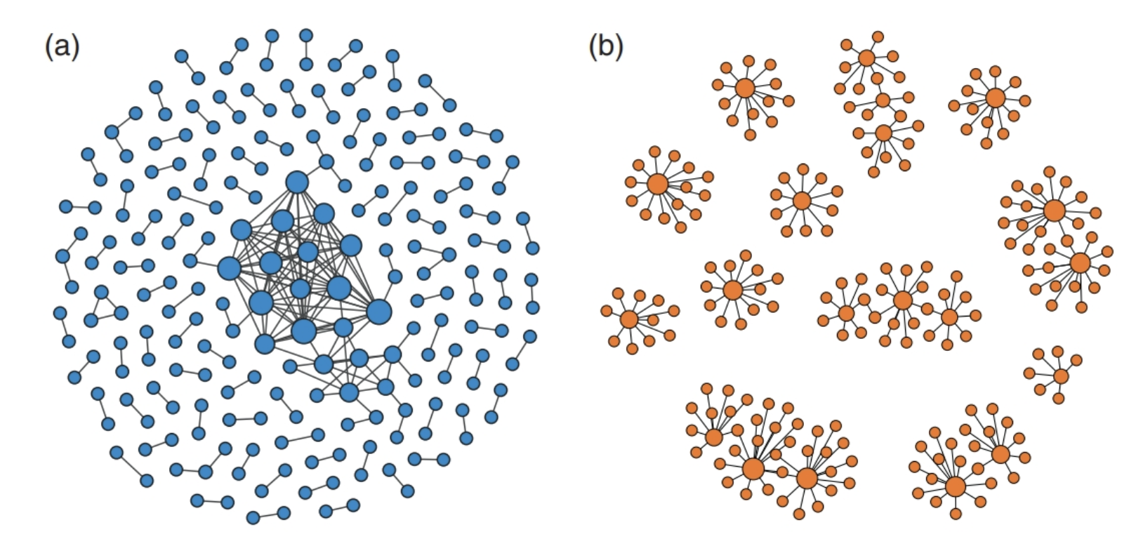
In social networks such as Facebook or Twitter, people with similar attributes are more likely to be friends or share common interests. In a network, nodes with similar attributes tend to be connected to each other. This tendency is called homophily. Homophilic networks are assortative networks. Being in an echo chamber might be dangerous resulting in segragation and polarization. In contrast, disassortative networks are networks where nodes with similar attributes are less likely to be connected. In disassortative networks, nodes with different attributes are more likely to be connected. We can calculate network assortativity based on a specific node attributes. For example, we can calculate network assortativity based on node degree. In this case, we are calculating degree assortativity (correlation). Assortative networks exhibit core periphery structure. In contrast, disassortative networks exhibit star like structure. Internet, biological networks are disassortative. Social networks are assortative.

similar concept: birds of a feather flock together

Code

r = nx.degree_assortativity_coefficient(disconnected_graph.subgraph(first_component))
print("Degree assortativity: {}".format(r))

Degree assortativity: -0.4999999999999988

Alt Text — Figure 1: a) assortative networks b) disassortative network Section 2 reference 1

References

1: Network science textbook

2: Jungnickel textbook