Introduction

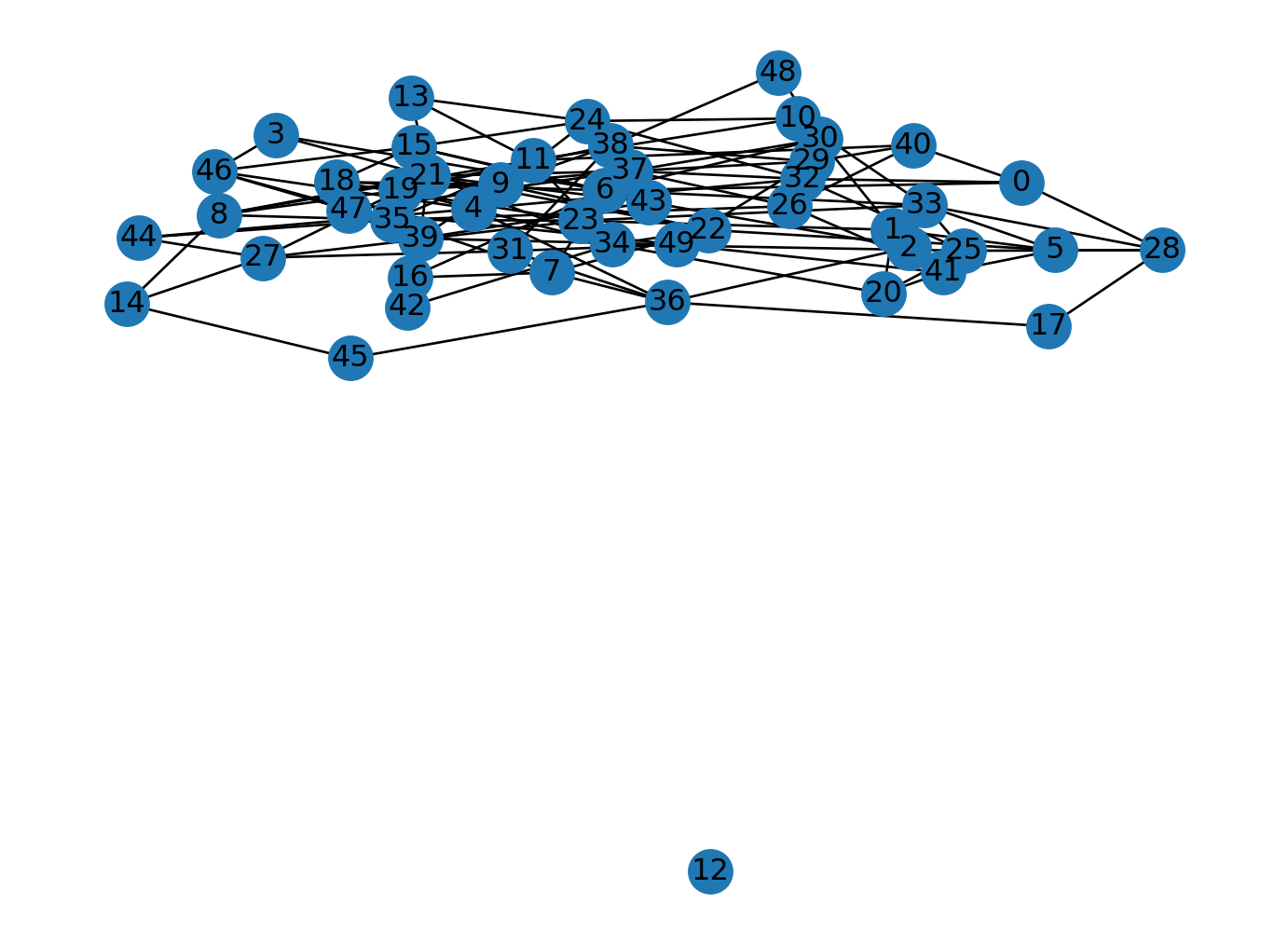
Many real networks share in common average short paths, high clustering(we can talk about this), and existence of few hub nodes that makes degree distribution heavy-tailed.

Graph generation (aka network models) can help us to understand the structure of the network. In this lecture, we will learn how to generate networks with different properties. We will also learn how to measure the robustness of the network. Generated graphs can be used as a benchmark to compare the performance of some network algorithms.

Erdos-Renyi Graphs

Erdos-Renyi graphs are random graphs. They are generated by randomly connecting nodes. The probability of connecting two nodes is \(p\). The probability of not connecting two nodes is \(1-p\). The probability of connecting two nodes is independent of other nodes. Erdos-Renyi graphs are also called \(G(n,p)\) graphs. \(n\) is the number of nodes and \(p\) is the probability of connecting two nodes.

Alt Text — Figure 1: Paul Erdos box. Courtesy of the reference 1.

How does the randomization work: 1. We start with a set of nodes. 2. We connect each pair of nodes with probability \(p\). That is we generate a random number between 0 and 1. If the random number is less than \(p\), we connect the pair of nodes. If the random number is greater than \(p\), we do not connect the pair of nodes. 3. We repeat step 2 for each pair of nodes.

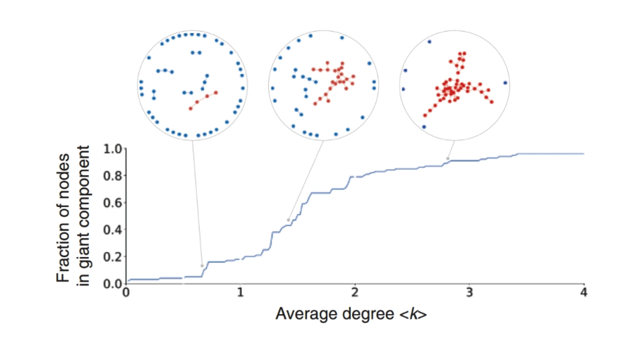
A giant component forms when the average degree is greater than 1.

Let’s generate an Erdos-Renyi graph with 50 nodes and \(p=0.1\).

Code

import networkx as nx
import matplotlib.pyplot as plt
import numpy as np
import random

n = 50
p = 0.1
G = nx.erdos_renyi_graph(n, p)
nx.draw(G, with_labels=True)
plt.show()

The next graph to generate is a \(G(n,m)\) graph. In this graph, we specify the number of nodes and the number of edges. The number of edges is \(m\). The probability of connecting two nodes is \(p=\frac{m}{\binom{n}{2}}\). Let’s generate a \(G(n,m)\) graph with 50 nodes and 50 edges.

Code

n = 50
m = 50
G = nx.gnm_random_graph(n, m)
nx.draw(G, with_labels=True)
plt.show()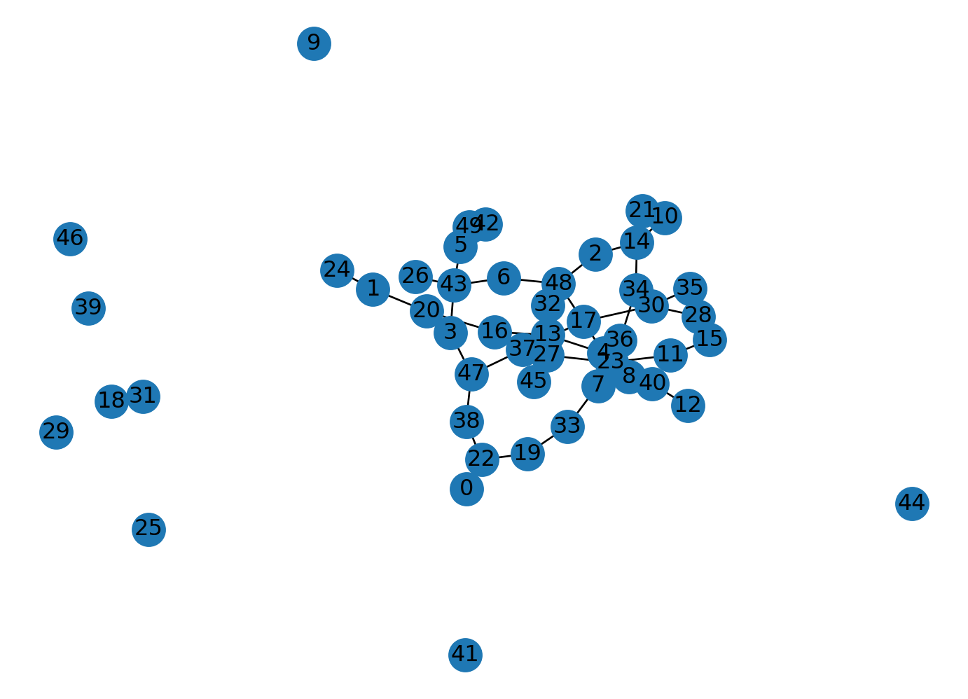

The link probability is correlated with the density of a random network. However, real networks are sparse therefore the link probability should be close to zero to model real networks.

Diameter of random networks turns out to be small. The average number of contacts a person can maintain is 150(see Dunbar’s number). At a distance of 5 the number of reachable people is \(150^5 \approx 75B\). This is more than the world population.

Triangles are rare in random networks. That brings the idea of networks models that generate networks with high clustering.

Watts-Strogatz Graphs

Watts-Strogatz graphs are small-world graphs. They are generated by randomly rewiring edges. Rewiring maintains high clustering while producing shorter paths. The probability of rewiring an edge is \(p\).

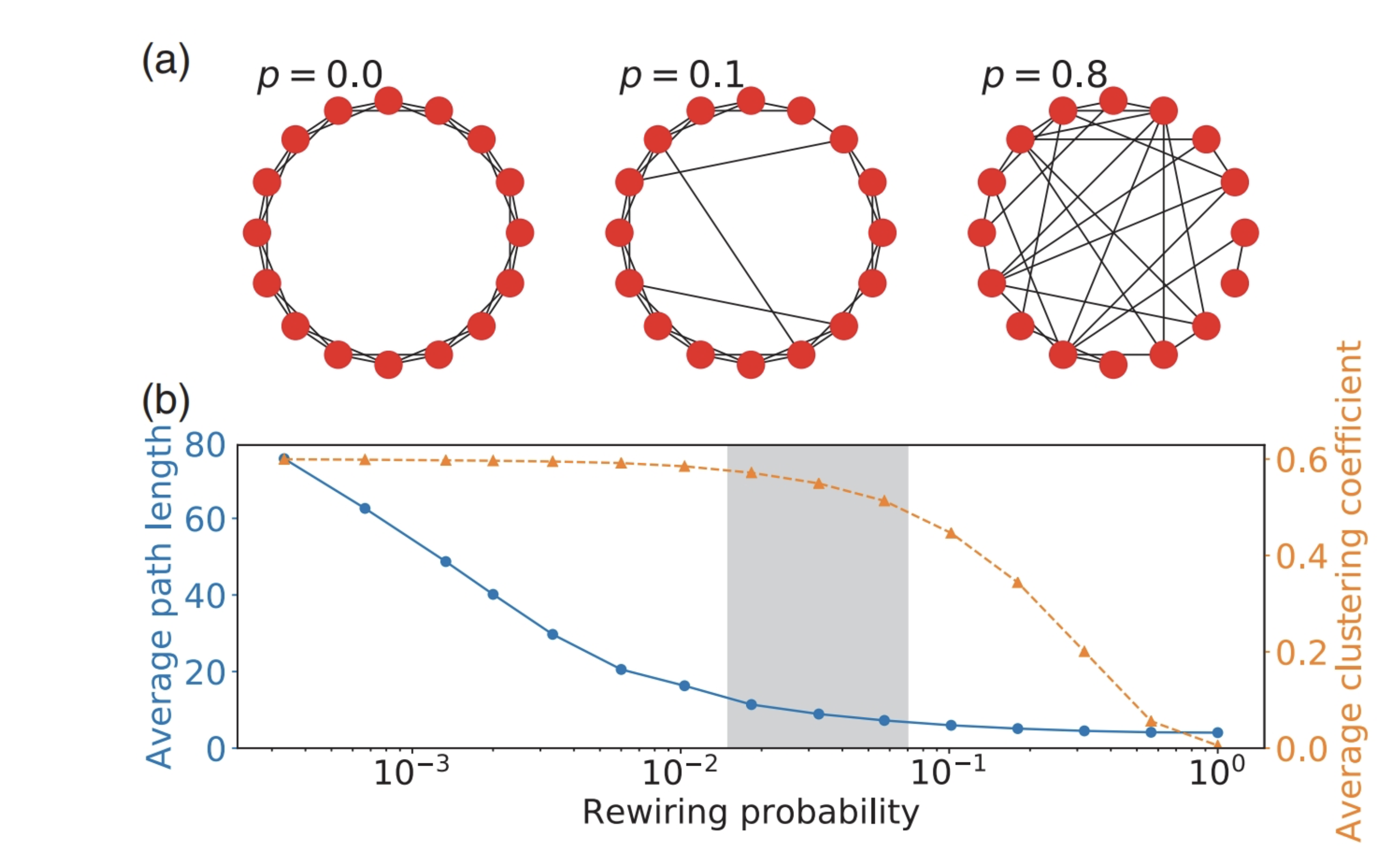
Let’s generate a Watts-Strogatz graph with 50 nodes, 10 edges, and \(p=0.1\).

Code

n = 50
k = 10
p = 0.1
G = nx.watts_strogatz_graph(n, k, p)
nx.draw(G, with_labels=True)
plt.show()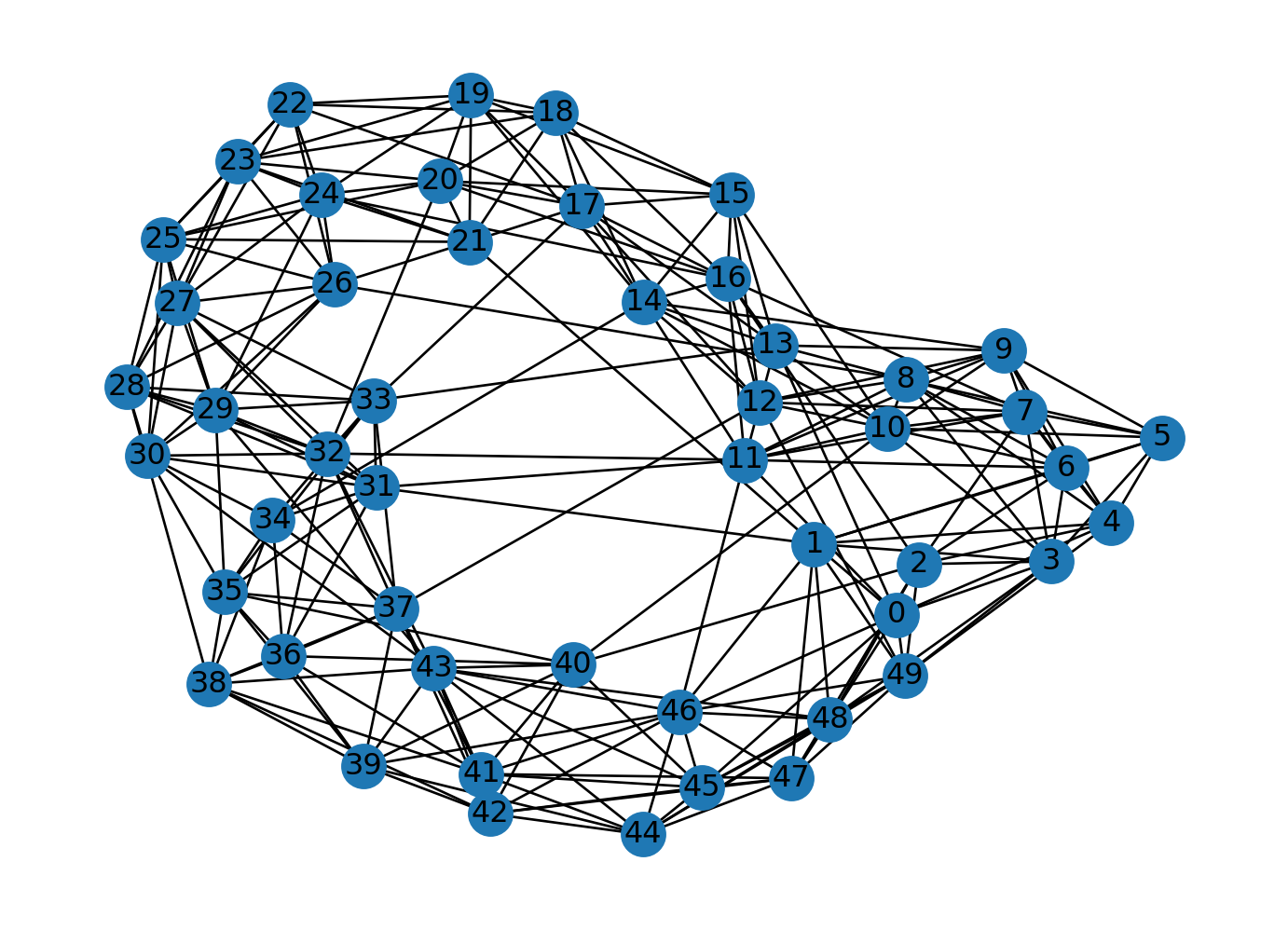

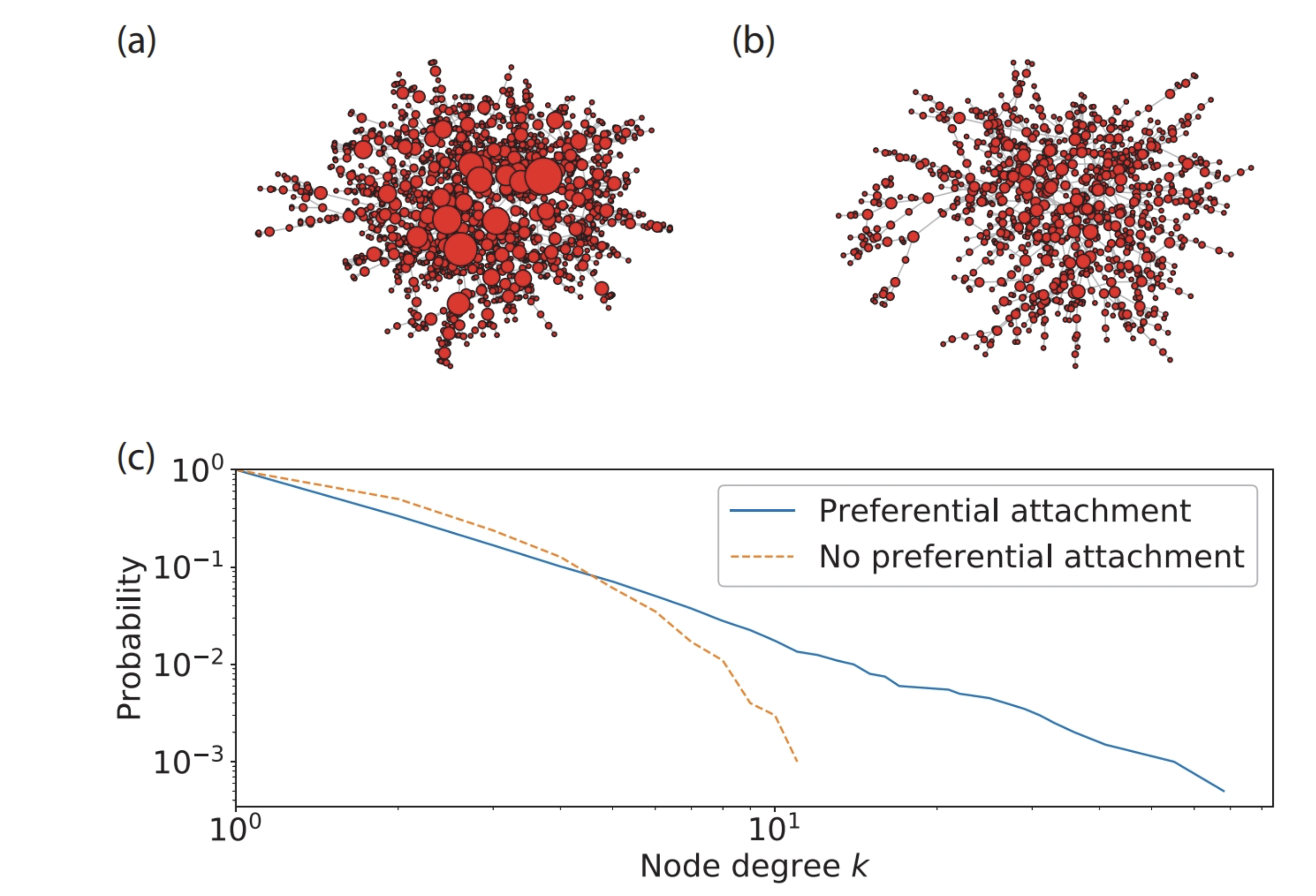
Barabasi-Albert Graphs

Barabasi-Albert graphs are scale-free graphs. This model is more relavant to dynamic networks as the context requires adding new nodes. They are generated by preferential attachment. The probability of connecting a new node to an existing node is proportional to the degree of the existing node. The more connected a node is, the more likely it is to be connected to a new node. Let’s generate a Barabasi-Albert graph with 50 nodes and 10 edges.

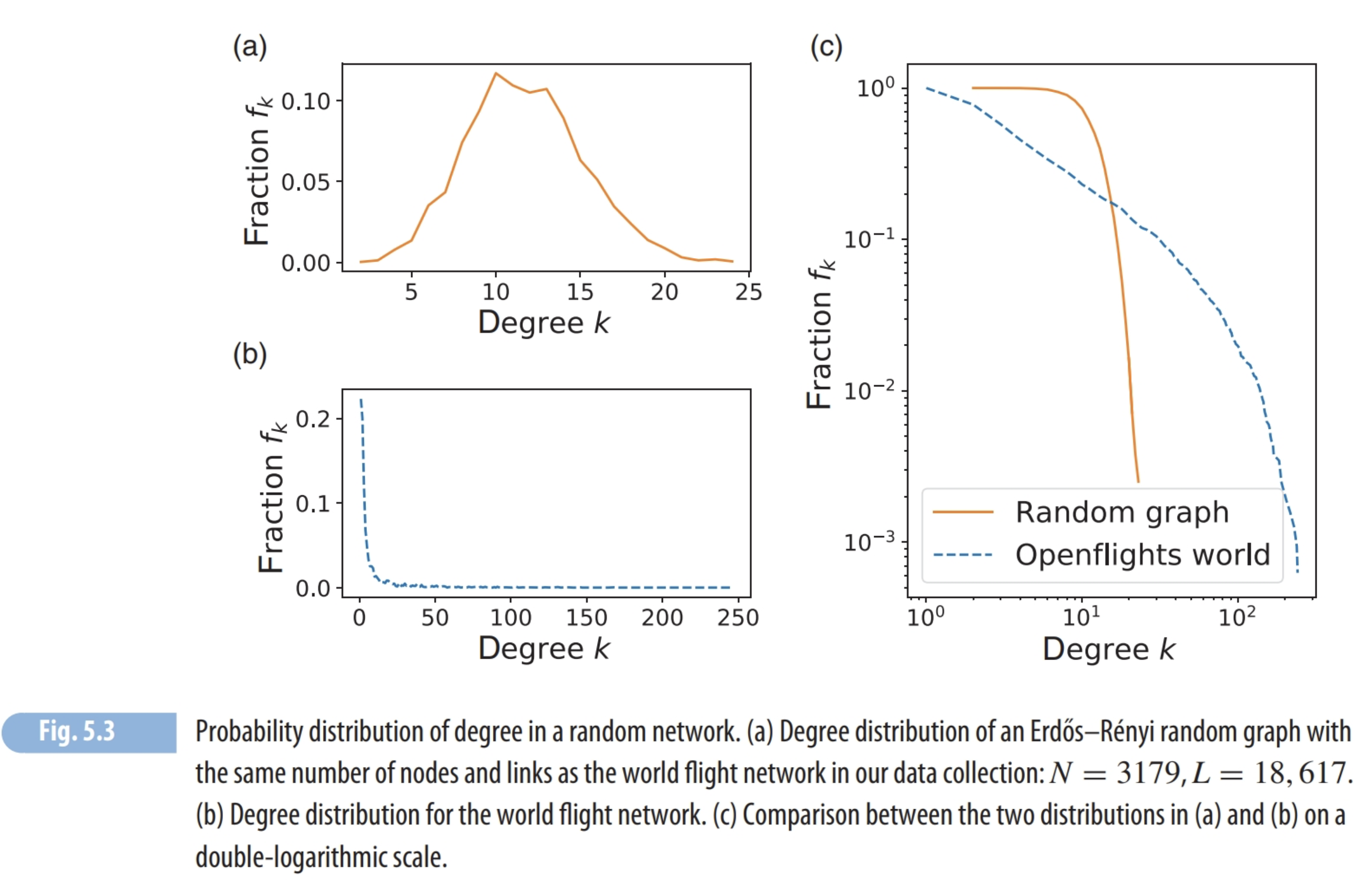
The probability that a node has degree \(k\) is proportional to \(k^{-\alpha}\). \(\alpha\) is a parameter that is usually between 2 and 3.

Code

import networkx as nx
n = 50
m = 3
G = nx.barabasi_albert_graph(n, m, seed=42)
#plot the graph using node sizes proportional to degree
nx.draw(G, with_labels=True, node_size=[v * 50 for v in dict(G.degree()).values()])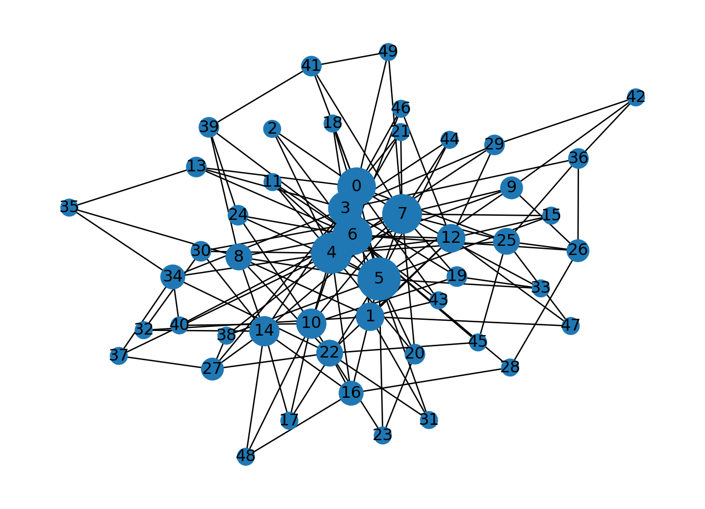

In order to understand how the preferential attachment works, let’s generate a Barabasi-Albert graph with 4 nodes and 5 edges. Let’s add a new node to the graph and create edges to existing nodes based on the probabilities.

Code

import networkx as nx
import numpy as np

# Let's create a small graph with 4 nodes and 4 edges
G = nx.DiGraph()
G.add_edge(1, 2)
G.add_edge(2, 3)
G.add_edge(2, 4)
G.add_edge(3, 4)
G.add_edge(4, 1)

# Calculate the probabilities based on the degree of each node.
degrees = np.array([G.degree(n) for n in G.nodes()])
probabilities = degrees / degrees.sum()

# Let's add a new node (5) to the graph and create edges to existing nodes based on the probabilities
i = 5
m = 2 # Number of edges to be added
new_edges = list(zip([i]*m, np.random.choice(G.nodes, size=m, replace=False, p=probabilities)))
G.add_edges_from(new_edges)

# Verify the graph
print(probabilities)
print(new_edges)
print(G.edges())

[0.2 0.3 0.2 0.3]
[(5, 2), (5, 4)]
[(1, 2), (2, 3), (2, 4), (3, 4), (4, 1), (5, 2), (5, 4)]

We can add more nodes to the system and create edges to existing nodes based on the probabilities.

Code

import networkx as nx
import matplotlib.pyplot as plt

# Number of initial nodes (minimum should be 2)
m0 = 3

# Number of nodes to add
m = 3

# Number of nodes
N = 12

# Create a graph with m0 nodes
G = nx.complete_graph(m0)

# Add nodes one by one
for i in range(m0, N):
    # Compute the sum of degrees of all nodes
    sum_degrees = sum(dict(G.degree()).values())
    
    # Create a list with probability of each node to connect to the new one
    probabilities = [float(G.degree(node)) / sum_degrees for node in G.nodes]
    
    # Add the new node connected to m nodes
    new_edges = list(zip([i]*m, np.random.choice(G.nodes, size=m, replace=False, p=probabilities)))
    G.add_edges_from(new_edges)

# Draw the graph
nx.draw(G, with_labels=True, node_size=[v * 100 for v in dict(G.degree()).values()])
plt.show()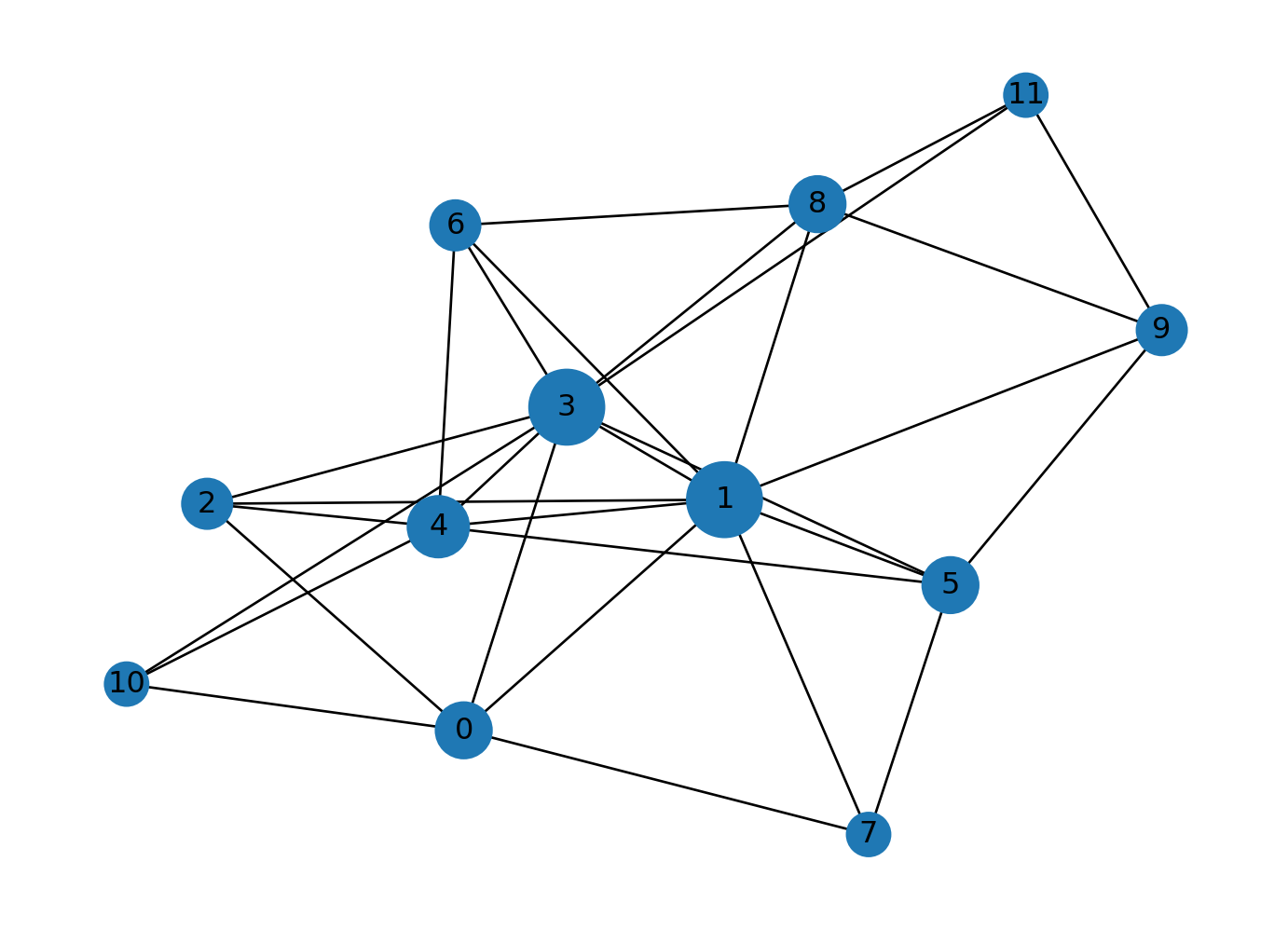

There is an excellent chapter to read about the scale-free property in the Scale-Free.

Robustness

Robustness is the ability of the network to maintain its functionality when some nodes or edges are removed. Robustness can be measured by the size of the largest connected component. The largest connected component is the largest subgraph that is connected. The size of the largest connected component is the number of nodes in the largest connected component. The size of the largest connected component is normalized by the number of nodes in the network. The normalized size of the largest connected component is called the giant component ratio. The giant component ratio is between 0 and 1. The giant component ratio is 1 when the network is fully connected. The giant component ratio is a measure of the robustness of the network. The higher the giant component ratio, the more robust the network is.

Let’s measure the robustness of the Erdos-Renyi graph that we generated earlier.

Code

n = 50
p = 0.1
G = nx.erdos_renyi_graph(n, p)
nx.draw(G, with_labels=True)
plt.show()

# Find the largest connected component
largest_connected_component = max(nx.connected_components(G), key=len)

# Calculate the ratio of nodes in the largest connected component to the total nodes in G
ratio = len(largest_connected_component) / len(G.nodes())

# Print the ratio
print("Ratio of nodes in largest connected component to total nodes:", ratio)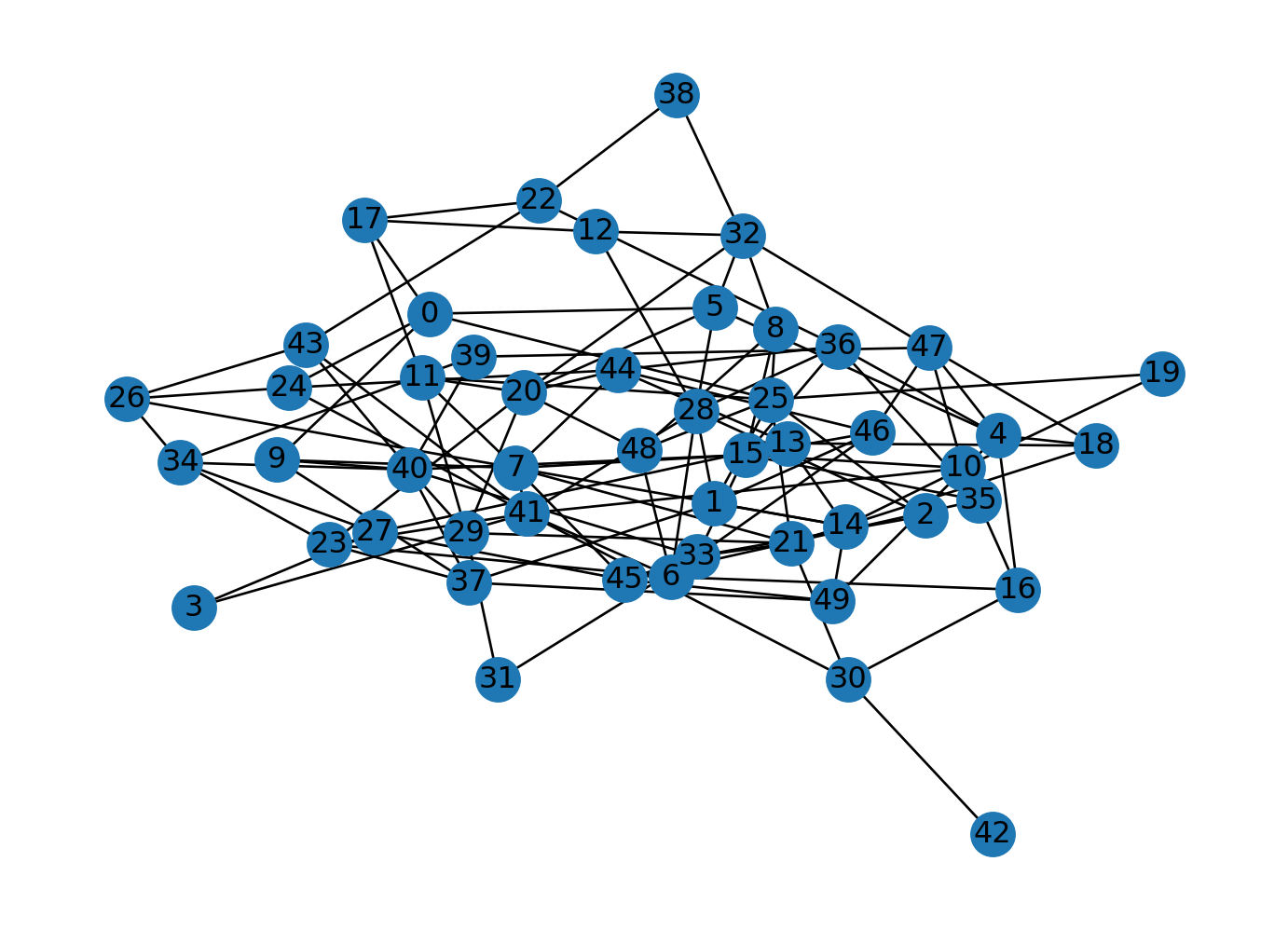

Ratio of nodes in largest connected component to total nodes: 1.0

Let’s measure the robustness of the Barabasi-Albert graph that we generated earlier.

Code

n = 50
m = 10
G = nx.barabasi_albert_graph(n, m)
nx.draw(G, with_labels=True)
plt.show()

# Find the largest connected component
largest_connected_component = max(nx.connected_components(G), key=len)

# Calculate the ratio of nodes in the largest connected component to the total nodes in G
ratio = len(largest_connected_component) / len(G.nodes())

# Print the ratio
print("Ratio of nodes in largest connected component to total nodes:", ratio)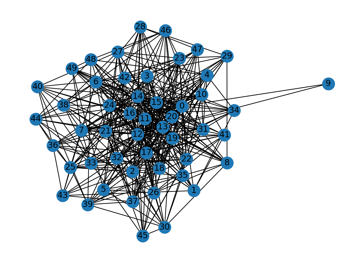

Ratio of nodes in largest connected component to total nodes: 1.0

Let’s measure the robustness of the Watts-Strogatz graph that we generated earlier.

Code

n = 50
k = 10
p = 0.1
G = nx.watts_strogatz_graph(n, k, p)
nx.draw(G, with_labels=True)
plt.show()

# Find the largest connected component
largest_connected_component = max(nx.connected_components(G), key=len)

# Calculate the ratio of nodes in the largest connected component to the total nodes in G
ratio = len(largest_connected_component) / len(G.nodes())

# Print the ratio
print("Ratio of nodes in largest connected component to total nodes:", ratio)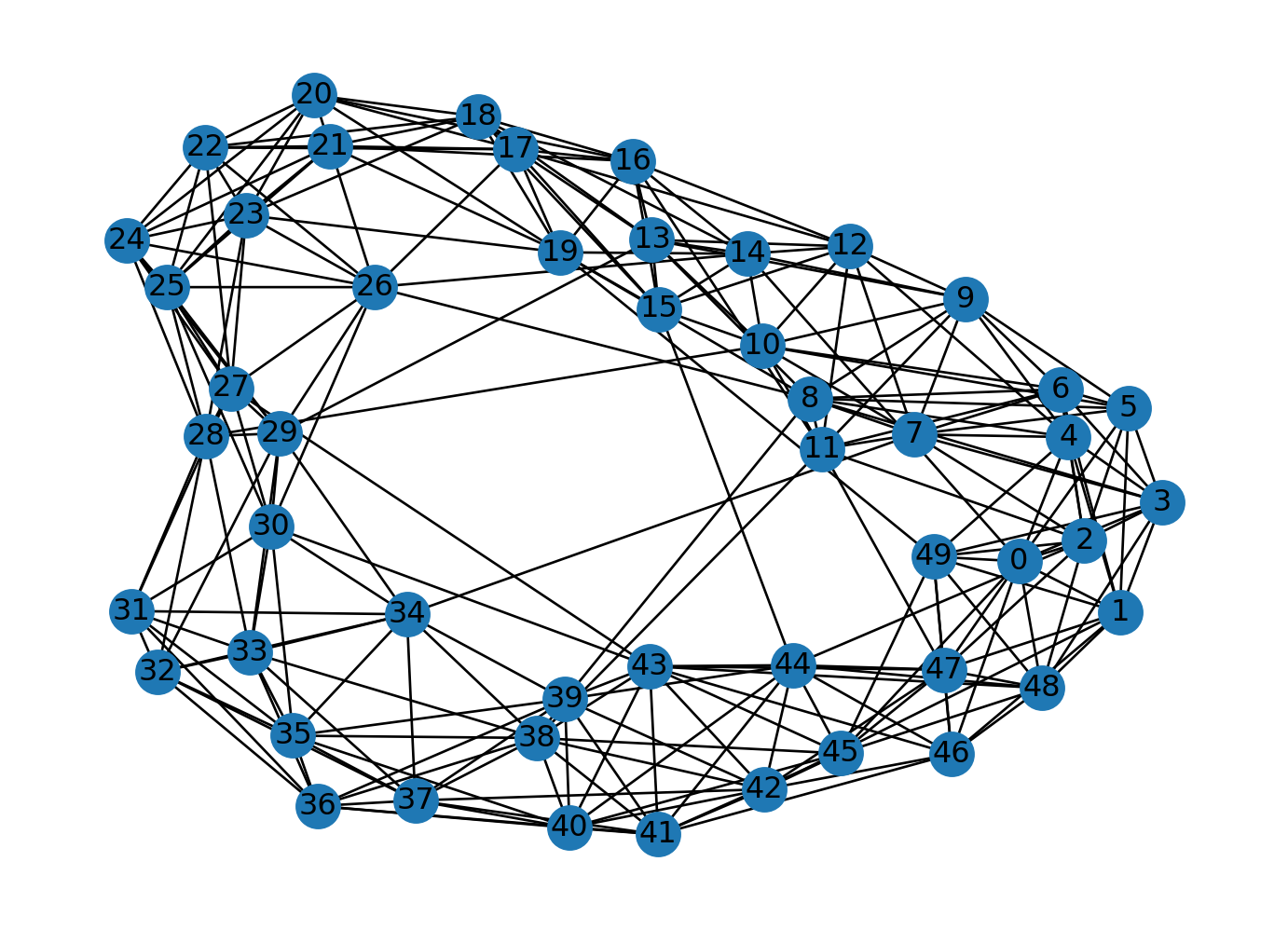

Ratio of nodes in largest connected component to total nodes: 1.0

We can generate networks combining several of them. Lets combine a clique, a lolipop, and a barbell graph. A lolipop graph is a clique connected to a path. A barbell graph is two cliques connected by a path. Let’s generate a lolipop graph with 7 nodes in the clique and 3 nodes in the path. Let’s generate a barbell graph with 5 nodes in each clique and 3 nodes in the path. Let’s combine the lolipop and the barbell graphs.

Code

lolipop = nx.lollipop_graph(7, 3)
nx.draw(lolipop, with_labels=True)
plt.show()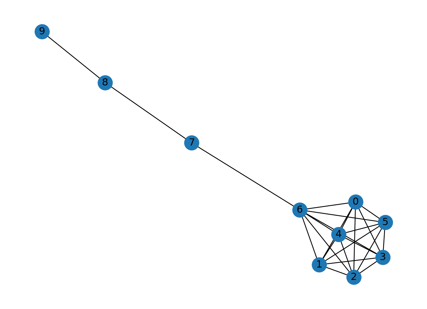

Code

barbell = nx.barbell_graph(5, 3)
nx.draw(barbell, with_labels=True)
plt.show()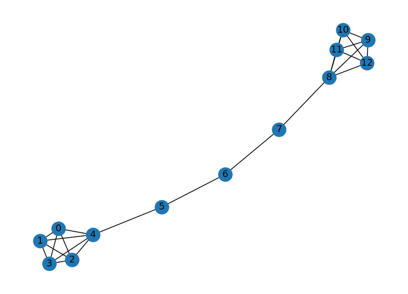

Code

def get_random_node(graph):
    return np.random.choice(graph.nodes)
allGraphs = nx.compose_all([lolipop,barbell])
allGraphs.add_edge(get_random_node(lolipop), get_random_node(barbell))
nx.draw(allGraphs, with_labels=True)
plt.show()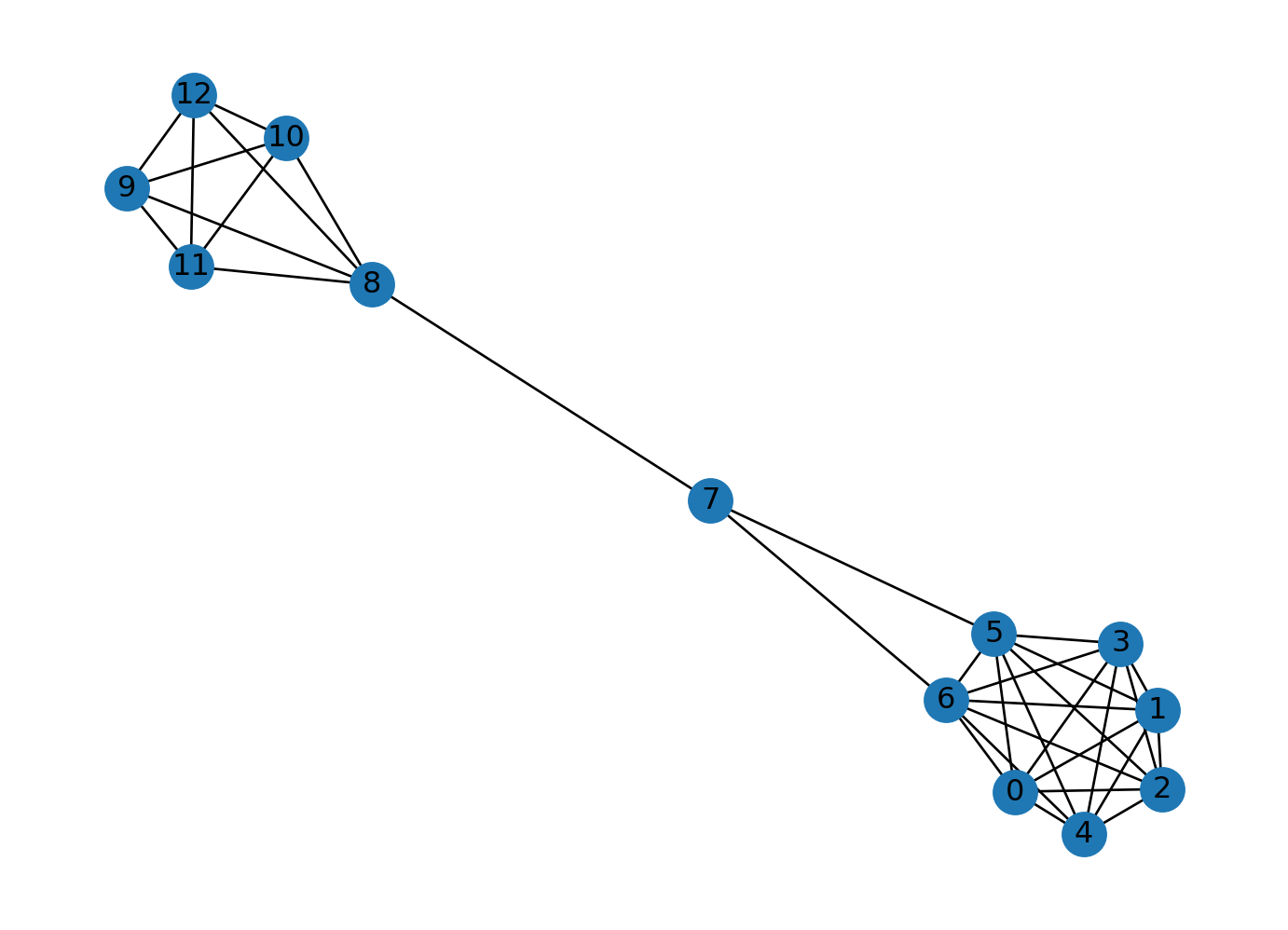

There are many other graph generators in the NetworkX library. You can find the list of graph generators in the NetworkX documentation.

Other robustness measures are also available. You can find the list of robustness measures in the NetworkX documentation.

There is a network robutness based on random and targeted attacks Python library. You can find the library in the GitHub repository.

Examples codes are provided below. Initial is the initial fraction of nodes in the largest connected component. Frac is the fraction of nodes in the largest component. Apl is the average shortest path length of the largest component.

Code

import networkx as nx
import matplotlib.pyplot as plt
from networkx_robustness import networkx_robustness

#Random NetworkX graph with 100 nodes
G = nx.gnp_random_graph(100, 0.5)

#Simulate a random attack on 20 nodes
initial, frac, apl = networkx_robustness.simulate_random_attack(G, attack_fraction=0.2)

#print the results
print(initial, frac, apl)

#plot fraction of nodes removed vs average path length
plt.plot(frac,apl)
#plt.show()

1.0 [0.99, 0.98, 0.97, 0.96, 0.95, 0.94, 0.93, 0.92, 0.91, 0.9, 0.89, 0.88, 0.87, 0.86, 0.85, 0.84, 0.83, 0.82, 0.81, 0.8] [1.5066996495567924, 1.5074689669682306, 1.5062285223367697, 1.5037280701754385, 1.503023516237402, 1.50354609929078, 1.5037400654511455, 1.504538939321548, 1.5054945054945055, 1.5076154806491886, 1.5071501532175688, 1.508881922675026, 1.5092221331194868, 1.508891928864569, 1.5095238095238095, 1.5083189902467011, 1.508374963267705, 1.5076784101174345, 1.5080246913580246, 1.5060126582278481]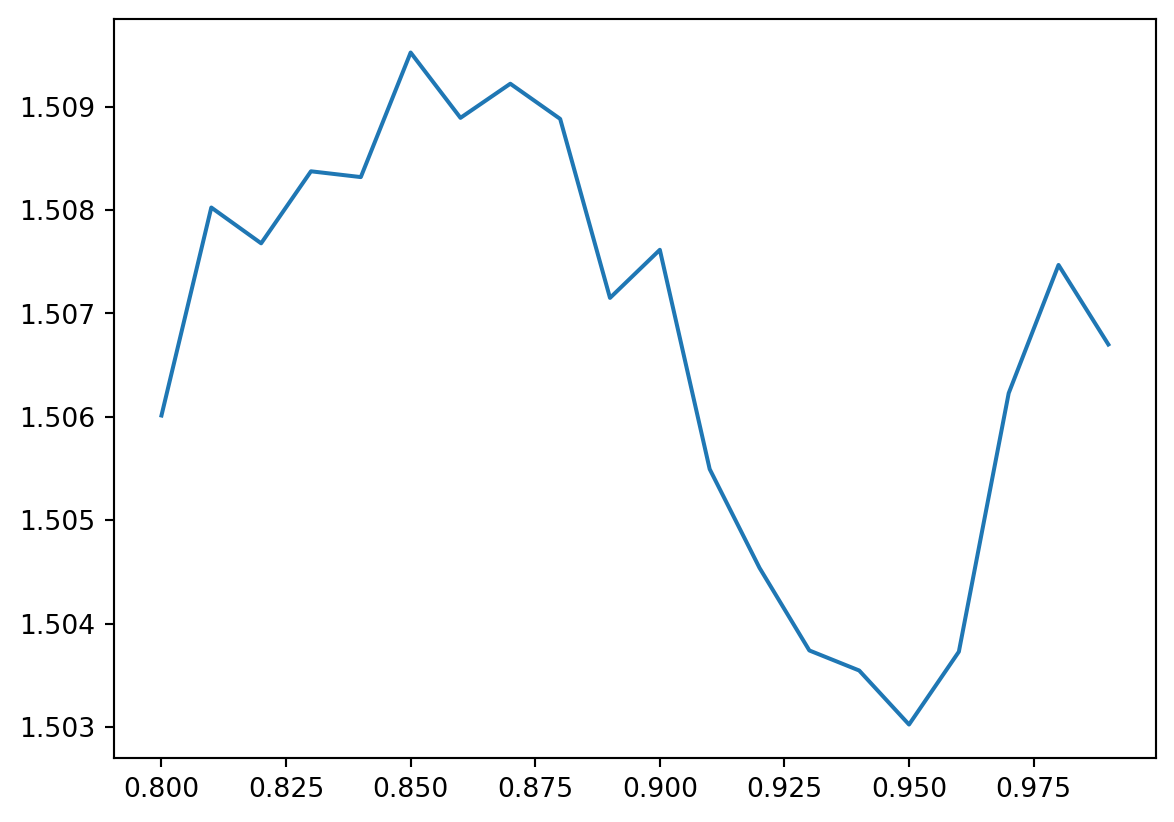

Code

from networkx_robustness import networkx_robustness
molloy_reed = networkx_robustness.molloy_reed(G)
print(molloy_reed)

49.33237704918033

Code

from networkx_robustness import networkx_robustness
CT = networkx_robustness.critical_threshold(lolipop)
print(CT)

None

Molloy-Reed Criterion (MR) states that a randomly wired network has a giant component if the degree distribution satisfies the following condition:

\(MR = \frac{<k^2>}{<k>}>2\)

Critical threshold (fraction of nodes to remove) to lose a giant component is:

\(1-\frac{1}{MR-1}\)

Robustness chapter in the Robustness is a good reference to read about robustness.

References

1: Network science textbook 2: NetworkX documentation 3: Barabasi Textbook