Introduction

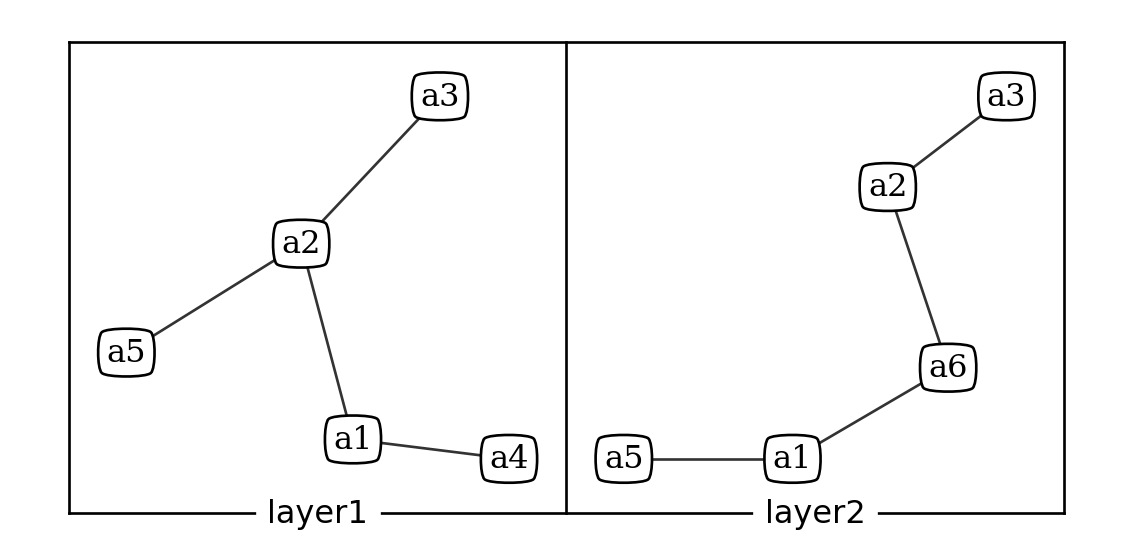
First introduced under social science domain, multilayer networks represented different type of relationships of the same nodes. The representation is now generalized to allow diffent nodes at each layer, different relathionships and connections between layers. Transportation networks, social networks, biological networks, and financial networks are examples of multilayer networks.

Alt Text — Figure 1: APS Dataset, paper collaborations in different subjects. Courtesy of the reference 1.

Mathematical Definition

I will be using the convention adopted in the first reference. We can define multilayer network

\(M = (Y, \vec{G}, G)\)

where \(Y\) is the set of layers, is the ordered list of networks, and \(G\) is the list of bipartite networks that represent relationships between pairs of layers.

Multiplex networks are multilayer networks where the set nodes is the same for all layers. They are also called replica nodes if interlinks are allowed between layers. Without interlinks a multiplex can be represented as

\(M = (Y, \vec{G})\)

where \(Y\) is the set of layers and is the ordered list of networks. Each network contains the same set of nodes.

Analyzing Multiplex Networks

One way of analyzing multiplex networks is flattening layers and analyzing the resulting single layer network. This approach is called single layer projection. Edge weights can be added to reflect the number of layers that contain the edge.

Actor Analysis

Degree standard deviation of an actor through layers is defined as

\(\sigma_{k} = \sqrt{\frac{1}{L-1}\sum_{\alpha=1}^{L}(k_{\alpha}-\bar{k})^2}\)

where \(k_{\alpha}\) is the degree of the actor in layer \(\alpha\), \(\bar{k}\) is the average degree of the actor, and \(L\) is the number of layers.

uunet Python package can be used to analyze multiplex networks. Detailed documentation and a tutorial can be found at uunet

Code

#install uunet
import uunet.multinet as ml
n = ml.read('tutorial/example1.txt')
ml.plot(n, vertex_labels_bbox = {"boxstyle":'round4', "fc":'white'})

Helper function defined to convert the output of the library to pandas dataframes.

Code

import pandas as pd
# transforms the typical output of the library (dictionaries) into pandas dataframes
def df(d):
  return pd.DataFrame.from_dict(d)

Use networkx objects as layers of the multiplex network

Code

import networkx as nx
l1 = nx.read_edgelist("tutorial/example_igraph1.dat")
l2 = nx.read_edgelist("tutorial/example_igraph2.dat")
n = ml.empty()
ml.add_nx_layer(n, l1, "layer1")
ml.add_nx_layer(n, l2, "layer2")
df( ml.edges(n) )

	from_actor	from_layer	to_actor	to_layer	dir
0	A	layer1	C	layer1	False
1	A	layer1	B	layer1	False
2	B	layer1	C	layer1	False
3	A	layer2	C	layer2	False

The library provides a multiplex mixture growth model based on some evolution functions. It’s limited to ER and PA models for now. A layer can grow internally or externally based on probabilities. If externally effected from other layers, dependency matrix can be used to define the dependency between layers.

Code

models_mix = [ ml.evolution_pa(3, 1), ml.evolution_er(100), ml.evolution_er(100) ]
pr_internal = [1, .2, 1]
pr_external = [0, .8, 0]
dependency = [ [1, 0, 0], [0.5, 0, 0.5], [0, 0, 1] ]
generated_mix = ml.grow(100, 150, models_mix, pr_internal, pr_external, dependency)
l = ml.layout_multiforce(generated_mix, gravity = [.5])
ver = ml.vertices(generated_mix)
deg = [ml.degree(generated_mix, [a], [l])[0] for a,l in zip(ver['actor'], ver['layer'])]
ml.plot(generated_mix, layout = l, vertex_labels=[], vertex_size=deg)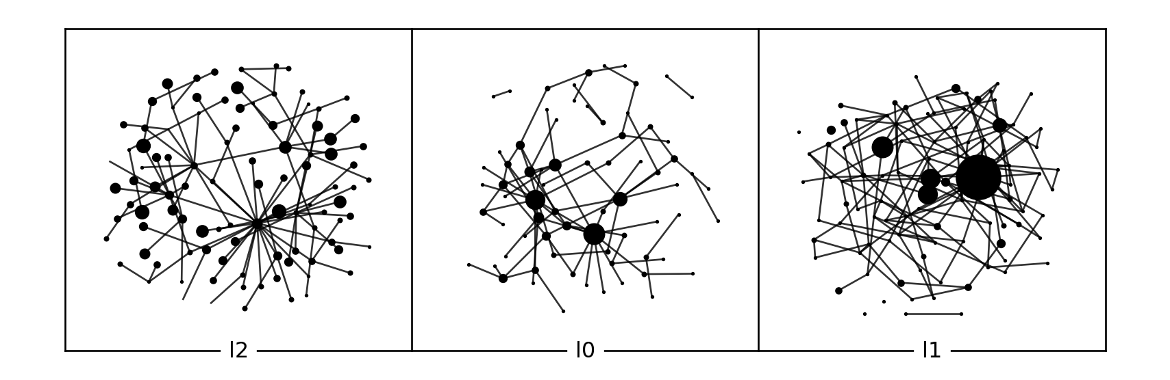

It is also possible to read existing datasets in the library.

Code

net = ml.data("aucs")
ml.layers(net)

['lunch', 'facebook', 'coauthor', 'leisure', 'work']

You can merge some layers into a single layer.

Code

ml.flatten(net, "offline", ['work', 'leisure', 'lunch'] )
ml.layers(net)

['lunch', 'facebook', 'coauthor', 'leisure', 'work', 'offline']

Code

net = ml.data("aucs")
l2 = ml.layout_multiforce(net, w_inter = [1], w_in = [1, 0, 0, 0, 0], gravity = [1, 0, 0, 0, 0])
ml.plot(net, layout = l2, grid = [2, 3], vertex_labels = [])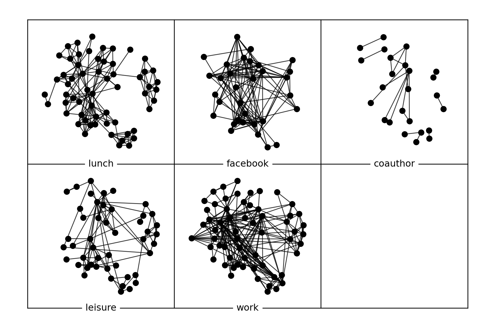

Some summary network metrics can be obtained from the library. \(n,m\) are number of nodes and edges, \(nc\) is number of components, \(slc\) is the size of larges component, \(dens\) is the density, \(cc\) is the average clustering coefficient, \(apl\) is the average shortest path length, \(dia\) is the diameter of the layer.

Code

df( ml.summary(net) )

	layer	n	m	dir	nc	slc	dens	cc	apl	dia
0	lunch	60	193	False	1	60	0.109040	0.568926	3.188701	7
1	facebook	32	124	False	1	32	0.250000	0.480569	1.955645	4
2	coauthor	25	21	False	8	6	0.070000	0.428571	1.666667	3
3	leisure	47	88	False	2	44	0.081406	0.343066	3.122622	8
4	work	60	194	False	1	60	0.109605	0.338786	2.390395	4

Other network statistics can be obtained converting multiplex object to networkx object.

Code

import networkx as nx
layers = ml.to_nx_dict(net)
nx.degree_assortativity_coefficient(layers["facebook"])

0.0027009183122244525

Layers can be compared in pairs based on difference/similarity of node/edge properties. The formulations are explained in the reference 3.

Code

comp = df( ml.layer_comparison(net, method = "jeffrey.degree") )
comp.columns = ml.layers(net)
comp.index = ml.layers(net)
comp

	lunch	facebook	coauthor	leisure	work
lunch	0.000000	0.420768	2.896653	1.328825	0.837241
facebook	0.420768	0.000000	2.021401	1.017798	0.710679
coauthor	2.896653	2.021401	0.000000	0.452108	0.591749
leisure	1.328825	1.017798	0.452108	0.000000	0.211845
work	0.837241	0.710679	0.591749	0.211845	0.000000

Code

df( ml.layer_comparison(net, method = "jaccard.actors") )

	0	1	2	3	4
0	1.000000	0.533333	0.416667	0.783333	0.967213
1	0.533333	1.000000	0.295455	0.519231	0.533333
2	0.416667	0.295455	1.000000	0.411765	0.416667
3	0.783333	0.519231	0.411765	1.000000	0.783333
4	0.967213	0.533333	0.416667	0.783333	1.000000

Code

df( ml.layer_comparison(net, method = "pearson.degree") )

	0	1	2	3	4
0	1.000000	0.312560	0.148637	0.281517	0.246475
1	0.312560	1.000000	0.547277	0.378174	0.540601
2	0.148637	0.547277	1.000000	0.480845	0.427194
3	0.281517	0.378174	0.480845	1.000000	0.068050
4	0.246475	0.540601	0.427194	0.068050	1.000000

Code

df( ml.layer_comparison(net, method = "jaccard.edges") )

	0	1	2	3	4
0	1.000000	0.178439	0.064677	0.277273	0.339100
1	0.178439	1.000000	0.058394	0.158470	0.186567
2	0.064677	0.058394	1.000000	0.101010	0.091371
3	0.277273	0.158470	0.101010	1.000000	0.205128
4	0.339100	0.186567	0.091371	0.205128	1.000000

Degrees and degree deviations of actors can be obtained.

Code

ml.degree(net, actors=['U4'])

[49]

Code

deg = ml.degree(net)
act = ml.actors(net)
list(act.values())[0]

degrees = [ [deg[i], list(act.values())[0][i]] for i in range(len(deg)) ]
degrees.sort(reverse = True)

degrees[0:5]

[[49, 'U4'], [47, 'U67'], [46, 'U91'], [44, 'U79'], [44, 'U123']]

Code

top_actors = []
for el in degrees[0:5]:
      top_actors.append( el[1] )

layer_deg = dict()
layer_deg["actor"] = top_actors
for layer in ml.layers(net):
    layer_deg[layer] = ml.degree(net, actors = top_actors, layers = [layer] )

df( layer_deg )

	actor	lunch	facebook	coauthor	leisure	work
0	U4	15	12	NaN	1.0	21
1	U67	12	13	NaN	2.0	20
2	U91	7	14	3.0	14.0	8
3	U79	13	15	NaN	7.0	9
4	U123	6	11	NaN	NaN	27

Code

deg_dev = dict()
deg_dev["actor"] = top_actors
deg_dev["dd"] = ml.degree_deviation(net, actors = top_actors)

df( deg_dev )

	actor	dd
0	U4	8.133880
1	U67	7.418895
2	U91	4.261455
3	U79	5.230679
4	U123	9.987993

Neigborhood centralities can be calculated. See the difference from degrees.

Code

ml.degree(net, actors = ["U4"], layers = ["work", "lunch"])
ml.neighborhood(net, actors = ["U91"], layers = ["facebook", "leisure"])

[22]

Neigborhood centrality exclusive to the queried layers can be calculated.

Code

ml.xneighborhood(net, actors = ["U91"], layers = ["facebook", "leisure"])

[13]

Relevance is the ratio between neighborhood centrality of the queried layers and all layers.

Code

layer_rel = dict()
layer_rel["actor"] = top_actors
for layer in ml.layers(net):
    layer_rel[layer] = ml.relevance(net, actors = top_actors, layers = [layer] )

df( layer_rel )

	actor	lunch	facebook	coauthor	leisure	work
0	U4	0.576923	0.461538	NaN	0.038462	0.807692
1	U67	0.521739	0.565217	NaN	0.086957	0.869565
2	U91	0.318182	0.636364	0.136364	0.636364	0.363636
3	U79	0.541667	0.625000	NaN	0.291667	0.375000
4	U123	0.206897	0.379310	NaN	NaN	0.931034

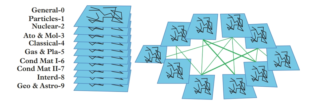
Multiplex networks are special cases of multilayer networks. Multilayer networks can be defined with different nodes at each layer. Pymnet libary can be used to visulaize and analyze multilayer networks.

Code

#!git clone https://github.com/bolozna/Multilayer-networks-library.git
#!pip install ./Multilayer-networks-library
import pymnet as pn
fig=pn.draw(pn.er(10,3*[0.4]),layout="spring", show=True)
fig.savefig("net.pdf")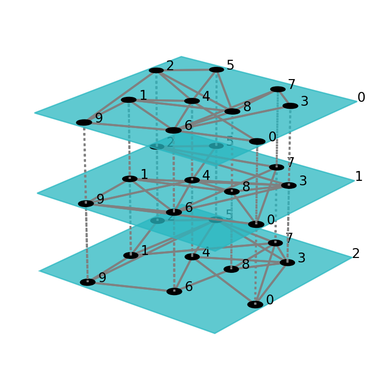

Code

gml = pn.er(10,3*[0.4])
#list(gml)
#list(gml.edges)
#list(gml.iter_layers())
#list(gml.iter_node_layers())
#list(gml[0,0])
#gml[0,0].deg()
#gml[0,0].str()
#pn.degs(gml)
#pn.density(gml)
#pn.cc_barrat(gml,(0,0))
#pn.multiplex_density(gml)
#pn.supra_adjacency_matrix(gml)
#help(pn.models)
#help(pn.netio)

References

1: Bianconi, Ginestra. Multilayer Networks. Available from: VitalSource Bookshelf, Oxford University Press Academic UK, 2018.

2: uunet Python library

3: Bródka, Piotr, et al. “Quantifying layer similarity in multiplex networks: a systematic study.” Royal Society open science 5.8 (2018): 171747.