First Words on Neural Networks (NNs) or Deep Learning Fundementals
What is a Neural Network?
A neural network is a computational model that is inspired by the way biological neural networks in the human brain process information. The key element of this model is the neuron, which is a mathematical function that takes an input and produces an output. The output is then passed to other neurons in the network. The network is composed of layers of neurons, with each layer performing a different type of computation. The neurons in each layer are connected to the neurons in the next layer by weights, which are parameters that determine the strength of the connection between neurons. The network learns by adjusting these weights based on the input data and the desired output.
Why Neural Networks?
Neural networks are capable of learning complex patterns in data.
They can be used to solve a wide range of problems, including image recognition, speech recognition, natural language processing, and game playing.
They have been shown to outperform traditional machine learning algorithms in many tasks.
They are highly flexible and can be adapted to different types of data and problems.
They are scalable and can be trained on large datasets using parallel computing.
Some of NN applications
Image recognition
Speech recognition
Natural language processing
Game playing
Robotics
Healthcare
Finance
Marketing
Transportation
Manufacturing
Energy
Brief history of NNs or DL
1943: McCulloch and Pitts propose a mathematical model of a neuron.
1958: Rosenblatt introduces the perceptron, a simple neural network model.
1969: Minsky and Papert show the limitations of perceptrons.
1986: Rumelhart, Hinton, and Williams introduce backpropagation, a method for training neural networks.
1990s: Neural networks fall out of favor due to limitations in training algorithms and computational power.
2006: Hinton and Salakhutdinov introduce deep belief networks, a precursor to modern deep learning.
2012: Krizhevsky, Sutskever, and Hinton win the ImageNet competition using a deep convolutional neural network.
2015: AlphaGo, a deep reinforcement learning system, defeats a human Go champion
2018: OpenAI’s GPT-2, a large language model, generates human-like text.
2020: DeepMind’s AlphaFold predicts protein structures with high accuracy.
DL Mathematics Basics (reference 2 )
Liear Algebra, Calculus, Probability and Statistics, and Optimization are the four main branches of mathematics that are used in deep learning.
Intro
NumPy is a popular library for linear algebra in Python. It provides support for arrays, matrices, and linear algebra operations such as matrix multiplication, matrix inversion, and eigenvalue decomposition. Below code defines an array from a list and prints its size and shape.
Code
import numpy as npa = np.array([1,2,3,4])a.sizea.shape# 2D array, list of lists is usedb = np.array([[1,2,3,4],[5,6,7,8]])print(b)b.shaped = np.array([[1,2,3],[4,5,6],[7,8,9]])print(d)d.shape
[[1 2 3 4]
 [5 6 7 8]]
[[1 2 3]
 [4 5 6]
 [7 8 9]]
(3, 3)
Some examples of modifing arrays are given below. : indicates all the elements along a specific dimension.
Code
#zeros and onesa = np.zeros((3,4), dtype="uint32")a[0,3] =42a[1,1] =66ab =11*np.ones((3,1))b#indexinga = np.arange(12).reshape((3,4)) #similar to python range functiona[1] #short for a[1,:]a[1] = [44,55,66,77]aa[:2] #short for a[:2,:]a[:2,:3] #first two rows and first three columnsb = np.arange(12)bb[::2] #every other elementb[::-1] #reversea = np.arange(24).reshape((4,3,2)) # collection of 3x2 matrices that is a 3D arrayaa[1,:,:] = [[11,22],[33,44],[55,66]] # second matrix is replacedaa[2,...] = [[99,99],[99,99],[99,99]] # third matrix is replaced, ... is used for the rest of the dimensions
SciPy uses NumPy under the hood. We can focus on stats module. Say test scores from two classes, how strongly can we believe that the same process generated these two sets of data? The t-test is a classic method for answering this question. One way to evaluate its result is to look at the p-value. A probability near 1 means we have a lot of confidence that the two sets are from the same process.
Code
import numpy as npfrom scipy.stats import ttest_ind # t-test for independent samplesa = np.random.normal(0,1,1000)b = np.random.normal(0,0.5,1000)c = np.random.normal(0.1,1,1000)ttest_ind(a,b) #notice a and be has the same averagettest_ind(a,c)
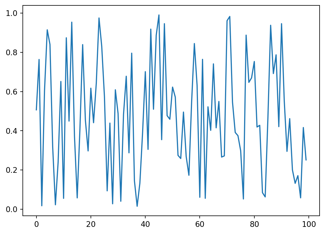
Matplotlib is popular for generating plots. We can plot NumPy arrays with it. Plot windows provides a way to interact with the plot.You can configure subplots for example.
Code
import numpy as npimport matplotlib.pyplot as pltx = np.random.random(100) # 100 random numbers between 0 and 1plt.plot(x)plt.show()
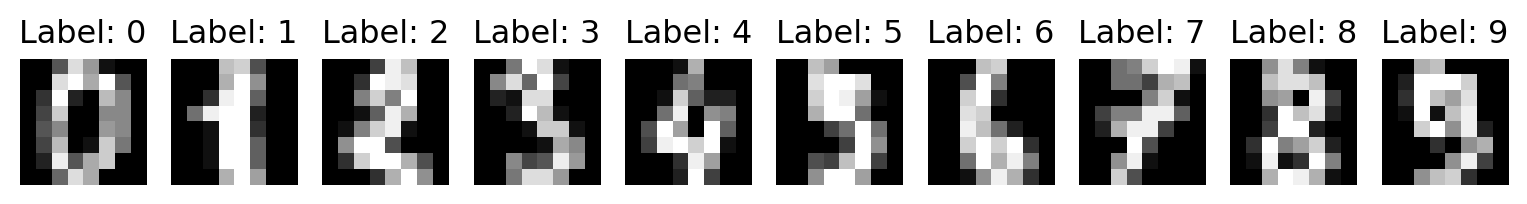
The famous Scikit-learn library is used for machine learning in Python. For our case, we can use it to build a simple neural network to classify small 8×8-pixel grayscale images of handwritten digits. This dataset is built into sklearn.
Code
import numpy as npfrom sklearn.datasets import load_digitsfrom sklearn.neural_network import MLPClassifierd = load_digits()digits = d["data"] #1,797 rows, with 64 columns per row, labels = d["target"] #you can name targets instead of labels. a vector of 1,797 digit labels.N =200#number of test samplesK =10# You can adjust this to visualize more or fewer digitsplt.figure(figsize=(10, 2)) # Adjust the figure size as neededfor i inrange(K): plt.subplot(1, K, i +1) plt.imshow(digits[i].reshape(8, 8), cmap='gray') plt.title(f"Label: {labels[i]}") plt.axis('off')plt.show()idx = np.argsort(np.random.random(len(labels))) #randomly shuffle the datax_test, y_test = digits[idx[:N]], labels[idx[:N]] #about 20 of each digit for testing.x_train, y_train = digits[idx[N:]], labels[idx[N:]] #approximately 160 images of each digit to train clf = MLPClassifier(hidden_layer_sizes=(128,)) #one hidden layer with 128 neurons, output layer size is deduced from y_train. This is called one instance of the model.clf.fit(x_train, y_train) #train the model. the learned weights and biases are in the model clf.score = clf.score(x_test, y_test)pred = clf.predict(x_test)err = np.where(y_test != pred)[0]print("score : ", score)print("errors:")print(" actual : ", y_test[err])print(" predicted: ", pred[err])# Print the weights and biasesprint("Weights between layers:")for i, coef inenumerate(clf.coefs_):print(f"Layer {i +1} to Layer {i +2} weights shape: {coef.shape}")print(coef)print("\nBiases for each layer:")for i, intercept inenumerate(clf.intercepts_):print(f"Layer {i +2} biases shape: {intercept.shape}")print(intercept)
What’s your accuracy? If you were to guess accurracy?
Probability
Each event is a sample from the sample space, and the sample space represents all the possible events. The sample space for the roll of a standard die is the set {1, 2, 3, 4, 5, 6}. If a feature input to a neural network can take on any value in the range [0, 1], then [0, 1] is the sample space for that feature. Probabilities always sum to 1.0 over all possible values of the sample space. Assume \(A_i\) represent an event i then we can use the summation of n events as follows:
\(\sum_{i=1}^{n} P(A_i) = 1\)
What if we roll two dice and sum them? The sample space is the set of integers from 2 through 12. By counting the ways events can happen and dividing by the total number of events, we can determine the probability. If you flip three coins simultaneously, what is the probability of getting no heads, one head, two heads, or three heads? We can enumerate the possible outcomes and see.
Code
import numpy as npN =1000000M=3heads = np.zeros(M+1) for i inrange(N): flips = np.random.randint(0,2,M) h, _ = np.bincount(flips, minlength=2) heads[h] +=1prob = heads / Nprint("Probabilities: %s"% np.array2string(prob))
Sum rule is applied to find the probability of the union of two events. The probability of the union of two events is the sum of the probabilities of the individual events minus the probability of their intersection. If the events are mutually exclusive, sun rule is formulated as follows:
\(P(A \cup B) = P(A) + P(B)\)
While sum rule tells us about A or B happening, product rule tells us about A and B happening. The probability of the intersection of two events is the product of the probabilities of the individual events. If the events are independent, product rule is formulated as follows:
\(P(A \cap B) = P(A)P(B)\)
If we have a dependent situation, the rule becomes:
\(P(A \cap B) = P(A)P(B|A)\)
Joint probability can be found using chain rule. Assume A,B,C are three random variables. The joint probability can be found as follows:
because the joint probability of both A and B doesn’t depend on which event we call A and which we call B, we can write the joint probability as:
\(P(A,B) = P(A|B)P(B) = P(B|A)P(A)\)
Dividing the expressions by P(A) we get the Bayes rule:
\(P(B|A) = \frac{P(A|B)P(B)}{P(A)}\)
Statistics
A statistic is a number that characterizes a sample of data. There are four types of data: nominal (categorical), ordinal, interval, and ratio.
Nominal data: Categories with no inherent order, such as colors or names. Qualitative data.
Ordinal data: Categories with an inherent order, such as rankings or ratings. Qualitative data.
Interval data: Numerical data with meaningful differences but no true zero point, such as temperature in Celsius. Quantitative data.
Ratio data: Numerical data with meaningful differences and a true zero point (means absense), such as weight or height. Quantitative data.
In DL one-hot encoding is used to convert categorical data into numerical data. For example, if we have a list of colors, we can convert them into a list of binary values.
Code
import numpy as npcolors = ["red", "green", "blue", "red", "green", "green"]unique_colors = np.unique(colors)one_hot = np.zeros((len(colors), len(unique_colors)))for i, color inenumerate(colors): one_hot[i, np.where(unique_colors == color)[0]] =1print(one_hot)
Summary statistics are used to make sense of the data. Mean, weighted mean, geometric mean, harmonic mean, and median are some of the summary statistics. Harmonic mean is used in DL to calculate F1 score that is the harmonic mean of precision and recall.
Correlation describes the associations between variables or features of a dataset. In ML,highly correlated features were undesirable, as they didn’t add any new information and only served to confuse the models. The entire art of feature selection was developed, in part, to remove this effect[2]. For DL, it is less critical to have uncorrelated features, as the network can learn to ignore redundant information.
Pearson correlation coefficient is used to measure the linear relationship between two variables. It ranges from -1 to 1. A value of 1 indicates a perfect positive linear relationship, -1 indicates a perfect negative linear relationship, and 0 indicates no linear relationship. The closer the correlation coefficient is to zero, either positive or negative, the weaker the correlation between the features [2]. The formula using the expected values is given below:
The Pearson correlation looks for a linear relationship, whereas the Spearman looks for any monotonic association between the inputs [2] using the ranks of the feature values.
Linear Algebra
A scalar has no dimensions, a vector has one, and a matrix has two. As you might suspect, we don’t need to stop there. A mathematical object with more than two dimensions is colloquially referred to as a tensor. A matrix is a tensor of order 2. A vector is an order-1 tensor, and a scalar is an order-0 tensor[2].
Code
t = np.arange(36).reshape((3,3,4)) #stack of 3x4 images for exampleprint(t[0]) #first imageprint(t[0,0]) #first row of first imageprint(t[0,0,0]) #first element of first row of first image
[[ 0  1  2  3]
 [ 4  5  6  7]
 [ 8  9 10 11]]
[0 1 2 3]
0
A bookshelf example to access a word of a particular book. Locate the shelf, book, page, line, and the word.
Code
w = np.zeros((9,9,9,9,9))w[4,1,2,0,1] #second word, first line, third page, second book, fifth shelf
0.0
we can treat a scalar (order-0 tensor) as an order-5 tensor, like this:
Code
t = np.array(42).reshape((1,1,1,1,1))print(t)t.shape
[[[[[42]]]]]
(1, 1, 1, 1, 1)
Element-wise multiplication on two matrices (a and b) is often known as the Hadamard product.
Code
a = np.array([[1,2,3],[4,5,6]])b = np.array([[7,8,9],[10,11,12]])c = a*bprint(c)
[[ 7 16 27]
 [40 55 72]]
Inner product also called dot product is found by:
Code
import numpy as npdef inner(a,b): s =0.0for i inrange(len(a)): s += a[i]*b[i]return sa = np.array([1,2,3,4]) b = np.array([5,6,7,8])print(inner(a,b))print(np.dot(a,b))print(a.dot(b))(a*b).sum()
or if vectors are interpreted geometrically, the dot product is the product of the magnitudes of the two vectors and the cosine of the angle between them:
The outer product appears as a mixing of two different embedding vectors. Embeddings are the vectors generated by lower layers of a network, for example, the next to last fully connected layer before the softmax layer’s output of a traditional convolutional neural network (CNN) [2].
If we want to multiplt matrices A and B to find C, the elements of C are found by taking the dot product of the rows of A and the columns of B.
\(C_{ij} = \sum_{k=1}^{n} a_{ik}b_{kj}\)
Code
def matrixmul(A,B): I,K = A.shape J = B.shape[1] C = np.zeros((I,J), dtype=A.dtype)for i inrange(I):for j inrange(J):for k inrange(K): C[i,j] += A[i,k]*B[k,j]return CA = np.array([[1,2,3],[4,5,6]])B = np.array([[7,8],[9,10],[11,12]])C = matrixmul(A,B)print(C)
[[ 58  64]
 [139 154]]
We can use a matrix to transform points between spaces. For example a matrix can map a point from 2D to 3D space.
An affine transformation maps a set of points into another set of points so that points on a line in the original space are still on a line in the mapped space. The transformation is [2]:
\(y = Ax + b\)
In fact, we can view a feedforward neural network as a series of affine transformations, where the transformation matrix is the weight matrix between the layers, and the bias vector provides the translation[2].
We can characterize a matrix B by how it maps vectors using the inner product between the mapped vector and the original vector[2]. B is positive definite if:
\(x^TBx > 0, \forall x \neq 0\)
B is positive semidefinite if:
\(x^TBx \geq 0, \forall x\)
B is negative definite if:
\(x^TBx < 0, \forall x \neq 0\)
B is negative semidefinite if:
\(x^TBx \leq 0, \forall x\)
B is indefinite if it is none of the above.
If a symmetric matrix is positive definite, then all of its eigenvalues are positive. Similarly, a symmetric negative definite matrix has all negative eigenvalues. Positive and negative semidefinite symmetric matrices have eigenvalues that are all positive or zero or all negative or zero, respectively [2].
A is a square matrix, v is a column vector and λ is a scalar. If Av = λv, then v is an eigenvector (eigen comes from German self) of A and λ is the corresponding eigenvalue. The vector, v, is mapped by A back into a scalar multiple of itself [2].
For n dimensional vector x, \(L_p\) norm is defined as:
\(||x||_p = (\sum_{i=1}^{n} |x_i|^p)^{1/p}\)
For p=2, the norm is called the Euclidean norm. For p=1, the norm is called the Manhattan norm. For p=\(\infty\), the norm is called the maximum norm.
L2-norm is calculated explicitly as:
\(||x||_2 = \sqrt{\sum_{i=1}^{n} x_i^2}\)
If we replace x by difference of two vectors, we treat norms as distance measures between the vectors. So, we can calculate the distance (Euclidean) between two vectors as:
\(||x-y||_2 = \sqrt{\sum_{i=1}^{n} (x_i-y_i)^2}\)
For example, weight decay, used in deep learning as a regularizer, uses the L2-norm of the weights of the model to keep the weights from getting too large [2].
We can calculate the variance of the features with respect to each other. Covariance matrix is used to calculate the variance of the features with respect to each other. The covariance matrix is a square matrix that contains the variances of the features along the diagonal and the covariances between the features off the diagonal. The covariance between two features is calculated as:
Assume each row of X is a feature vector. n dimensional point in the space is represented by a row vector. Principal component analysis (PCA) is a technique to learn the directions of the scatter in the dataset, starting with the direction aligned along the greatest scatter. This direction is called the principal component[2]. The PCA steps are summarized as follows:
Subtract the mean from the data (mean centering).
Calculate the covariance matrix.
Calculate the eigenvectors and eigenvalues of the covariance matrix.
Sort the eigenvectors by their eigenvalues in decreasing order.
Project the data onto the eigenvectors (using the transformation matrix that has the eigenvectors).
Code
#download iris dataset, 150 samples, 4 featuresfrom sklearn.datasets import load_irisiris = load_iris().data.copy() #mean centeringm = iris.mean(axis=0)ir = iris - m#covariance matrix 4x4cv = np.cov(ir, rowvar=False) #eigenvalues and eigenvectorsval, vec = np.linalg.eig(cv)#sort by eigenvaluesval = np.abs(val)idx = np.argsort(val)[::-1]#fraction explained, eigenvalues proportional to variance along each eigenvector(PC)ex = val[idx] / val.sum()print("fraction explained: ", ex)#projection of data onto eigenvectors, keep first 2 components since they explain 98% of the variance#w is 2x4, d is 150x2w = np.vstack((vec[:,idx[0]],vec[:,idx[1]]))d = np.zeros((ir.shape[0],2)) for i inrange(ir.shape[0]): d[i,:] = np.dot(w,ir[i])
During PCA, you may lose a critical feature allowing class separation. As with most things in machine learning, experimentation is vital [2].
A more compact code for PCA is given below:
Code
from sklearn.decomposition import PCApca = PCA(n_components=2)d = pca.fit_transform(ir)
Sigular Value Decomposition (SVD)
For deep learning, you’ll most likely encounter SVD when calculating the pseudoinverse of a nonsquare matrix [2]. A matrix A (mxn) can be decomposed into three matrices U(mxm), Σ(mxn), and V(nxn), where U and V are orthogonal matrices and Σ is a diagonal matrix. The diagonal elements of Σ are the singular values of A. The SVD is given as:
\(A = U \Sigma V^T\)
The “singular” in “singular value decomposition” comes from the singular values of the matrix A. The singular values are the square roots of the positive eigenvalues of the matrix AAT.
Code
from scipy.linalg import svda = np.array([[3,2,2],[2,3,-2]])u,s,vt = svd(a)print(u)
SVD can be used to find principal components or pseudoinverse of a matrix that is not a square one. we can calculate the pseudoinverse of any general matrix as follows:
\(A^+ = V \Sigma^+ U^T\)
where Σ+ is the pseudoinverse of Σ. The pseudoinverse of a diagonal matrix is the reciprocal of the diagonal elements. If the diagonal element is zero, the reciprocal is zero.
Code
A = np.array([[3,2,2],[2,3,-2]])u,s,vt = svd(A)Splus = np.array([[1/s[0],0],[0,1/s[1]],[0,0]])Aplus = vt.T @ Splus @ u.Tprint(Aplus)print(A @ Aplus @ A)
The chain rule is used to find the derivative of a composite function. If y = f(g(x)), then the derivative of y with respect to x is given by:
\(\frac{dy}{dx} = \frac{dy}{du} \frac{du}{dx}\)
where u = g(x). The chain rule is used in backpropagation to calculate the gradient of the loss function with respect to the weights of the network.
Minima or maxima of functions are called extrema of a function. Dervatives at these points are zero. We can use the derivative as a pointer to tell us how to move closer and closer to the extrema. This is what gradient descent does…[2].
Gradients tell us the direction and magnitude of the change in the function value at a point. The direction of the maximum change in a function at any point is the gradient at that point [2]. Recall, the gradient is a vector field, so each point on the xy-plane has an associated vector pointing in the direction of the greatest change in the function value[2].
Optimization
Training a neural network is, to a first approximation, an optimization problem—the goal is to find the weights and biases leading to a minimum in the loss function landscape[2].
A first order optimization algorithm uses the gradient of the loss function to update the weights and biases. The simplest first order optimization algorithm is gradient descent. The update rule for gradient descent is given as:
\(w_{t+1} = w_t - \alpha \nabla L\)
where \(w_t\) is the weight at time t, α is the learning rate, and ∇L is the gradient of the loss function. The learning rate is a hyperparameter that controls the size of the update to the weights. If the learning rate is too large, the weights may oscillate around the minimum or even diverge. If the learning rate is too small, the weights may take a long time to converge to the minimum.
Let’s find the derivative of the weights and bias value for a single node of a hidden layer in a feedforward network[2].
Outputs of the previous layer, x, multiplied by the weights, w, and added to the bias, b, are passed through an activation function, such as ReLU, to get the output of the node, y. In order to apply backpropagation we need derivatives of y with respect to w and b. y is given as:
\(y = ReLU(wx + b)\)
Derivative of this function with respect to w is given as:
1-derivative of the dot product of w and x with respect to w is x. 2-derivative of the ReLU function is 1 if the input is positive and 0 otherwise.
Now, chain rule can be applied that is derivative of y with respect to w equals derivative of y with respect to z times derivative of z with respect to w where z is w.x + b and y is ReLU(z). Same logic can be applied to find the derivative of y with respect to b.
Training a deep neural network is, fundamentally, an optimization problem, so the potential utility of the Jacobian and Hessian is clear, even if the latter can’t be easily used for large neural networks[2].