Introduction to Decision Science (Operations Research)

What is Operations Research?

Operations Research (OR) is the discipline of applying advanced analytical methods to help make better decisions. OR is very often described as the science of better. Recently, there are suggestions within the community to change the name of the discipline to Decision Science. Here is the link to the article Distinguishing the Profession of Operations Research in the Age of Analytics, Big Data, Data Science and AI that discusses the name change.

Some examples of OR applications

• Scheduling of airline crews, trains, buses, etc.
• Design of production facilities
• Planning of production/inventory
• Design of supply chains
• Design of healthcare systems
• Design of transportation systems
• Design of sports schedules

Brief history of OR

• OR emerged as a distinct discipline during World War II.
• Research into military operations was conducted by scientists from a variety of fields.

Modeling basics

Modeling is the process of creating a simplified representation of a real-world situation that can be analyzed to make decisions. Representaion of a reality. Remember the famous quote by George Box: “All models are wrong, but some are useful.”

Some examples of Models

• A map
• A scale model of a building
• A mathematical equation
• A computer simulation
• A statistical model such as a regression model
• An optimization model

Deterministic vs. stochastic models

Linear vs. nonlinear models

Continuous vs. discrete models

Bold ones are dealt in this course.

Deterministic optimization models are also called mathematical programming models. Programming means planning in this context. Mathematical programming models have the following components:

• Decision variables (unknowns)
• Objective function (a measure of effectiveness in terms of the decision variables)
• Constraints (limitations on the decision variables or linear combinations of them). Constraints are two types: main constraints and variable domain constraints. Parameters are the data of the model.

In this course, we will assume that the parameters are known or we will use machine learning techniques to estimate them.

Refering to the textbook example Two Crude Petroleum (see lecture notes in pdf), decision variables are \(x_1\) and \(x_2\), objective function is \(f(x_1,x_2)\), and constraints are \(g_1(x_1,x_2)\) and \(g_2(x_1,x_2)\).

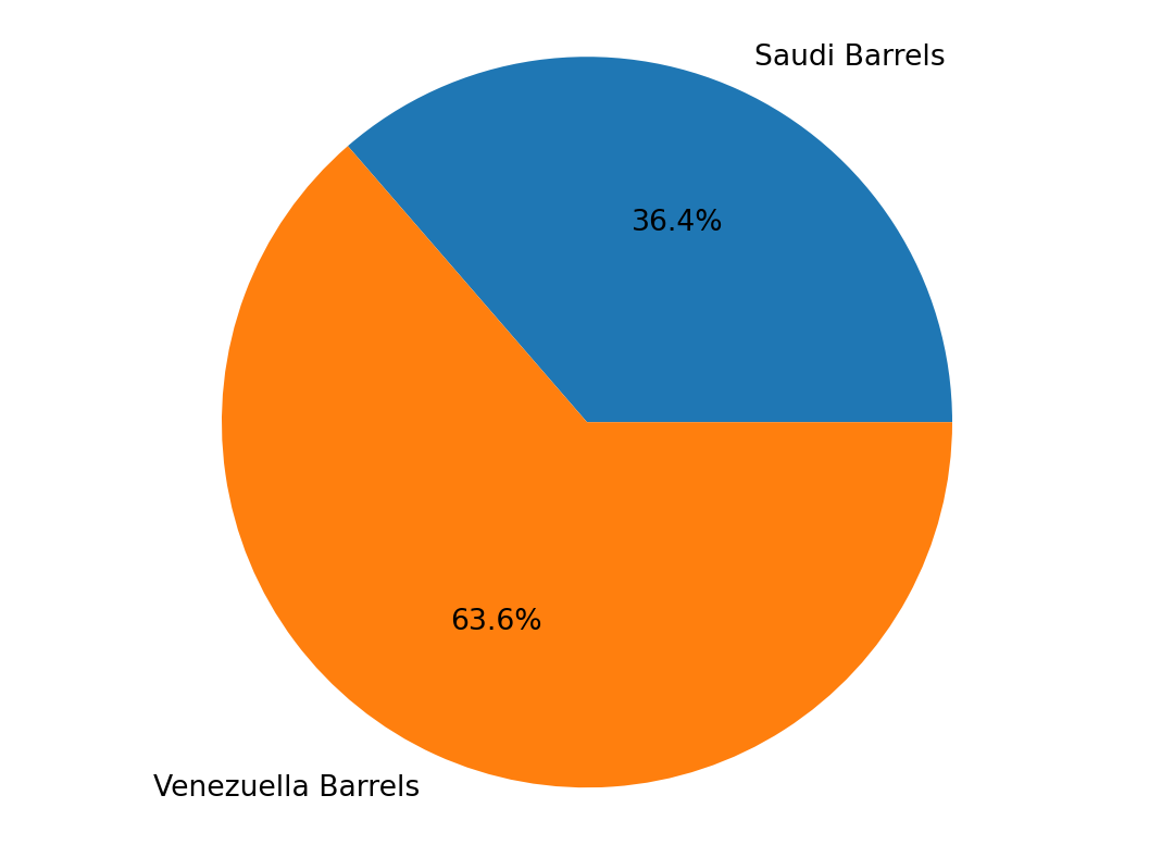
\(x_1\) = number of barrels (in thousands) of crude petrolem from Saudi Arabia to be purchased

\(x_2\) = number of barrels (in thousands) of crude petrolem from Venezuella to be purchased

The objective function is the total cost of purchasing crude petroleum from Saudi Arabia and Venezuella. The constraints are the total amount of crude petroleum purchased from Saudi Arabia and Venezuella should be at most 9000, 6000 barrels respectively and satify the demand of gasoline, jet fuel, and lubricants.

The two crudes differ in chemical composition and thus yield different product mixes. Each barrel of Saudi crude yields 0.3 barrel of gasoline, 0.4 barrel of jet fuel, and 0.2 barrel of lubricants. On the other hand, each barrel of Venezuelan crude yields 0.4 barrel of gasoline but only 0.2 barrel of jet fuel and 0.3 barrel of lubricants. The remaining 10% of each barrel is lost to refining. Saudi Arabia charges \$100 per barrel, and Venezuela charges \$75 per barrel. The demand for gasoline, jet fuel, and lubricants is 2000, 1500, and 500 barrels, respectively.

Decide (remember OR is decision science) how many barrels of crude petroleum to purchase from Saudi Arabia and Venezuella to minimize the total cost of purchasing crude petroleum.

Mathematical programming model

\[ \begin{align*} \text{min} \quad & 100x_1 + 75x_2 & \text{(total cost)} \\ \text{s.t.} \quad & 0.3x_1 + 0.4x_2 \geq 2.0 & \text{(gasoline requirement)} \\ & 0.4x_1 + 0.2x_2 \geq 1.5 & \text{(jet fuel requirement)} \\ & 0.2x_1 + 0.3x_2 \geq 0.5 & \text{(lubricant requirement)} \\ & x_1 \leq 9 & \text{(Saudi availability)} \\ & x_2 \leq 6 & \text{(Venezuelan availability)} \\ & x_1, x_2 \geq 0 & \text{(nonnegativity)} \end{align*} \]

AMPL model of the problem is given below. We will learn how to solve this model during a colab session.

Code

%pip install -q amplpy matplotlib pandas
from amplpy import AMPL, ampl_notebook

ampl = ampl_notebook(
    modules=["cbc", "highs"],  # modules to install
    license_uuid="your license number here",  # license to use
)  # instantiate AMPL object and register magics

[notice] A new release of pip is available: 24.0 -> 24.2
[notice] To update, run: /Library/Developer/CommandLineTools/usr/bin/python3 -m pip install --upgrade pip
Note: you may need to restart the kernel to use updated packages.
Please provide a valid license UUID. You can use a free https://ampl.com/ce license.

/Users/harunpirim/Library/Python/3.9/lib/python/site-packages/urllib3/__init__.py:35: NotOpenSSLWarning: urllib3 v2 only supports OpenSSL 1.1.1+, currently the 'ssl' module is compiled with 'LibreSSL 2.8.3'. See: https://github.com/urllib3/urllib3/issues/3020
  warnings.warn(

Code

%%ampl_eval
#decision variables
reset;
var x1 >= 0;
var x2 >= 0;

Code

%%ampl_eval
#objective function
minimize cost: 100 * x1 + 75 * x2;

Code

%%ampl_eval
#constraints
gasoline: 0.3 * x1 + 0.4 * x2 >= 2;
jetfuel: 0.4 * x1 + 0.2 * x2 >= 1.5;
lubricant: 0.2 * x1 + 0.3 * x2 >= 0.5;
avail_saudi: x1 <= 9;
avail_venez: x2 <= 6;

Code

# exhibit the model that has been built
#ampl.eval("show;")
#ampl.eval("expand;")
# solve using two different solvers
ampl.option["solver"] = "cbc"
ampl.solve()
ampl.option["solver"] = "highs"
ampl.solve()
ampl.display("_varname", "_var")
# create pandas series for production and raw materials
import pandas as pd
purchase = pd.Series(
    {
        "Saudi Barrels": ampl.get_value("x1"),
        "Venezuella Barrels": ampl.get_value("x2"),
    }
)
# display pandas series
display(purchase)
# create a pie chart
import matplotlib.pyplot as plt
plt.pie(purchase, labels=purchase.index, autopct="%1.1f%%")
plt.axis("equal")
plt.show()

cbc 2.10.10: cbc 2.10.10: optimal solution; objective 462.5
0 simplex iterations
 
HiGHS 1.6.0: HiGHS 1.6.0: optimal solution; objective 462.5
0 simplex iterations
0 barrier iterations
 
: _varname  _var    :=
1   x1       2
2   x2       3.5
;

Saudi Barrels         2.0
Venezuella Barrels    3.5
dtype: float64

References

1: Optimization in OR textbook by R. Rardin

2: AMPL Python Book