Quantitative Sensitivity Analysis
Introduction
The primal model is the main application of interest. ‘’The dual corresponding to a given primal formulation is a closely related LP with decision variables and constraints that quantify the sensitivity of primal results to changes in its parameters.’’[1]. There is one dual variable for each primal constraint and they quantify the sensitivity of the primal objective function to changes in the right-hand side of the corresponding primal constraint. The optimal dual variables are the shadow prices associated with the constraints.
Quantitative Sensitivity Analysis
Dual Variable Types
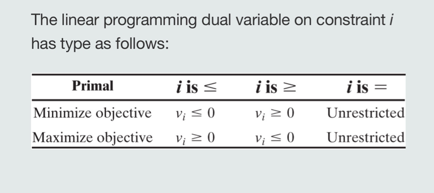
When we increase the RHS of supply constraints (\(\leq\)) the solution space is relaxed and the objective function value stays the same or improves (decrease for minimization, increase for maximization). That implies (for maximization) that the dual variable associated with the supply constraint is positive. When we decrease the RHS of supply constraints, the solution space is tightened and the objective function value stays the same or worsens. That implies that the dual variable associated with the supply constraint is negative (for maximization).
When we increase the RHS of demand constraints (\(\geq\)) the solution space is tightened and the objective function value stays the same or worsens. That implies that the dual variable associated with the demand constraint is negative. When we decrease the RHS of demand constraints, the solution space is relaxed and the objective function value stays the same or improves. That implies that the dual variable associated with the demand constraint is positive.
Figure 1 illustrates the dual variable types for supply and demand constraints.
See example 6.10 in the textbook for a detailed example.
‘Dual variables provide implicit prices for the marginal unit of the resource modeled by each constraint as its right-hand-side limit is encountered.’[1]
See example 6.11 in the textbook for a detailed example.
‘An activity’s (decision variable) non-zero constraint coefficients can be interpreted as amounts consumed or created per unit of the activity. By summing those coefficients times the implicit price \(v_i\) of the resources involved (dual varible corresponding to the \(i^{th}\) constraint), we can obtain an implicit marginal value (minimize problems) or price (maximize problems) for the entire activity.’[1]
Main Dual Constraints to Enforce Activity Pricing
‘Dual variables in a minimize (cost) problem would overvalue an activity if they priced it above its true cost coefficient \(c_j\). An activity implicitly worth more than it costs at optimality should be used in greater quantity. But then we would be improving on an optimal solution—an impossibility. Similarly for maximize (benefit) problems, we would want to reject any \(v_i\) s that priced the net value of resources that an activity uses below its real benefit \(b_j\). Otherwise, it too would yield an improvement on an already optimal solution.’[1]
Assuming non-negative activities, we can formulate the following constraints to enforce activity pricing:
\(c_j - \sum_{i=1}^{m} v_i a_{ij} \geq 0, \quad j=1,2,...,n\)
For maximization problems, we can formulate the following constraints to enforce activity pricing:
\(\sum_{i=1}^{m} v_i a_{ij} - b_j \geq 0, \quad j=1,2,...,n\)
See example 6.13 in the textbook for a detailed example.
The primal optimal solution is feasible for the dual problem and the dual optimal solution is feasible for the primal problem. The optimal objective function values of the primal and dual problems are equal. This is known as the strong duality theorem. We can write the following equations to show the strong duality theorem:
\(\sum_{j=1}^{n} c_j x_j = \sum_{i=1}^{m} b_i v_i\)
See example 6.14 in the textbook for a detailed example.
Primal Complemantary Slackness
The primal complementary slackness conditions are as follows:
\(v_i > 0 \Rightarrow \sum_{j=1}^{n} a_{ij} x_j = b_i\) \(v_i = 0 \Rightarrow \sum_{j=1}^{n} a_{ij} x_j \neq b_i\)
See example 6.15 in the textbook for a detailed example.
Dual Complemantary Slackness
The dual complementary slackness conditions are as follows:
\(x_j > 0 \Rightarrow \sum_{i=1}^{m} v_i a_{ij} = c_j\) \(x_j = 0 \Rightarrow \sum_{i=1}^{m} v_i a_{ij} \neq c_j\)
See example 6.16 in the textbook for a detailed example.
Generalizing Primal vs Dual Relationships
Assume \(i\) is the index for primal constraints and \(j\) is the index for primal decision variables. The primal maximization problem is as follows:
\(\max \sum_{j=1}^{n} c_j x_j\)
Corresponding dual problem is as follows:
\(\min \sum_{i=1}^{m} b_i v_i\)
If main constraints are \(\leq\) type, then the dual variable is \(v_i \geq 0\). If main constraints are \(\geq\) type, then the dual variable is \(v_i \leq 0\). If main constraints are \(=\) type, then the dual variable is \(v_i\) is free (URS).
If primal variables are non-negative, corresponding dual constraints are as follows:
\(c_j - \sum_{i=1}^{m} v_i a_{ij} \leq 0, \quad j=1,2,...,n\)
If primal variables are free, corresponding dual constraints are as follows:
\(c_j - \sum_{i=1}^{m} v_i a_{ij} = 0, \quad j=1,2,...,n\)
If primal variables are non-positive, corresponding dual constraints are as follows:
\(c_j - \sum_{i=1}^{m} v_i a_{ij} \geq 0, \quad j=1,2,...,n\)
The primal minimization problem is as follows:
\(\min \sum_{j=1}^{n} c_j x_j\)
Corresponding dual problem is as follows:
\(\max \sum_{i=1}^{m} b_i v_i\)
If main constraints are \(\leq\) type, then the dual variable is \(v_i \leq 0\). If main constraints are \(\geq\) type, then the dual variable is \(v_i \geq 0\). If main constraints are \(=\) type, then the dual variable is \(v_i\) is free (URS).
If primal variables are non-negative, corresponding dual constraints are as follows:
\(\sum_{i=1}^{m} v_i a_{ij} - c_j \leq 0, \quad j=1,2,...,n\)
If primal variables are free, corresponding dual constraints are as follows:
\(\sum_{i=1}^{m} v_i a_{ij} - c_j = 0, \quad j=1,2,...,n\)
If primal variables are non-positive, corresponding dual constraints are as follows:
\(\sum_{i=1}^{m} v_i a_{ij} - c_j \geq 0, \quad j=1,2,...,n\)
Computer Outputs
We consider two types of sensitivity analysis. One if constraint sensitivity and the other one is variable sensitivity analysis.
Constraint Sensitivity Analysis
Right handside ranges (usually denoted by down and up names) in the constraint sensitivity outputs show the interval within which the corresponding dual variable value provives the rate of change in the optimal value per unit change in RHS given that all other data held constant.
Variable Sensitivity Analysis
Objective function coefficient ranges (usually denoted by down and up names) in the variable sensitivity outputs show the interval within which the optimal primal variable value stays the same.
What Ifs
Dropping a constraint can change the optimal solution only if the constraint is active at optimality.
Adding a constraint can change the optimal solution only if that optimum violates the constraint.
An LP variable can be dropped without changing the optimal solution only if its optimal value is zero.
A new LP variable can change the current primal optimal solution only if its dual constraint is violated by the current dual optimum.
Refer to the colab notebook for a detailed example on how to use AMPL for sensitivity analysis.
References
1: Optimization in OR textbook by R. Rardin