Graphic Solutions of Linear Programming Problems

Solving Linear Progragramming (LP) problems

There are famous algorithms to solve LP problems. However, before learning those algorithms, we will learn how to solve LP problems graphically. That gives a good intuition about the problem and the solution. Graphic solution is limited to solve problems with 2 or three variables. In real life applications, an LP model can have millions of variables and constraints! Before getting hands on the graphical solutions, let’s practice one more modeling from your textbook:

Example 2.1: Formulating Formal Optimization Models

Given an equipment yard to be enclosed by a rectengular fence of at most 80 meters, what would the choice of lengt and width to find the maximum area?

Remember first step is to define the decision variables. Then, define the objective function and the constraints.

Decision Variables

• \(x_1\): Length of the fence
• \(x_2\): Width of the fence

Objective Function

• \(maximize \quad z = x_1 \times x_2\) (z is usually used for the name of the objective function)

Constraints

• \(2(x_1 + x_2) \leq 80\) (Perimeter constraint)

Model

\[\begin{aligned}maximize \ x_{1}\cdot x_{2}\\ subject \ to\\ 2\left( x_{1}+x_{2}\right) \leq 80\\ x_{1},x_{2}\geq 0\end{aligned}\]

This is not an LP model because the objective function is not linear. However, we used this example for the purpose of modeling.

Graphical Solution of an LP Problem

Let’s solve the two crude example using graphical solution. The LP model was:

\[ \begin{align*} \text{min} \quad & 100x_1 + 75x_2 & \text{(total cost)} \\ \text{s.t.} \quad & 0.3x_1 + 0.4x_2 \geq 2.0 & \text{(gasoline requirement)} \\ & 0.4x_1 + 0.2x_2 \geq 1.5 & \text{(jet fuel requirement)} \\ & 0.2x_1 + 0.3x_2 \geq 0.5 & \text{(lubricant requirement)} \\ & x_1 \leq 9 & \text{(Saudi availability)} \\ & x_2 \leq 6 & \text{(Venezuelan availability)} \\ & x_1, x_2 \geq 0 & \text{(nonnegativity)} \end{align*} \]

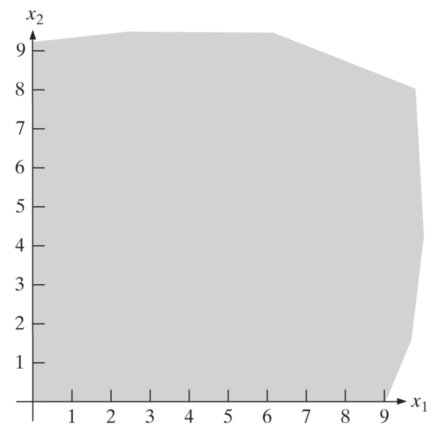
We need to plot the feasible solution space that satisfies all the constraints. Then, we need to find the optimal solution by moving the objective function line. Let’s start with the variable domain constraints that is \(x_1 \geq 0\) and \(x_2 \geq 0\). The feasible solution space is shown in the following figure:

Figure 1: feasible solution space. Courtesy of reference 1

Now, in addition to \(x_1 \geq 0\) and \(x_2 \geq 0\) constraints we will add a third one that is \(0.3x_1 + 0.4x_2 \geq 2.0\). The feasible solution space is shown in the following figure:

Figure 2: feasible solution space, new constraint added. Courtesy of reference 1

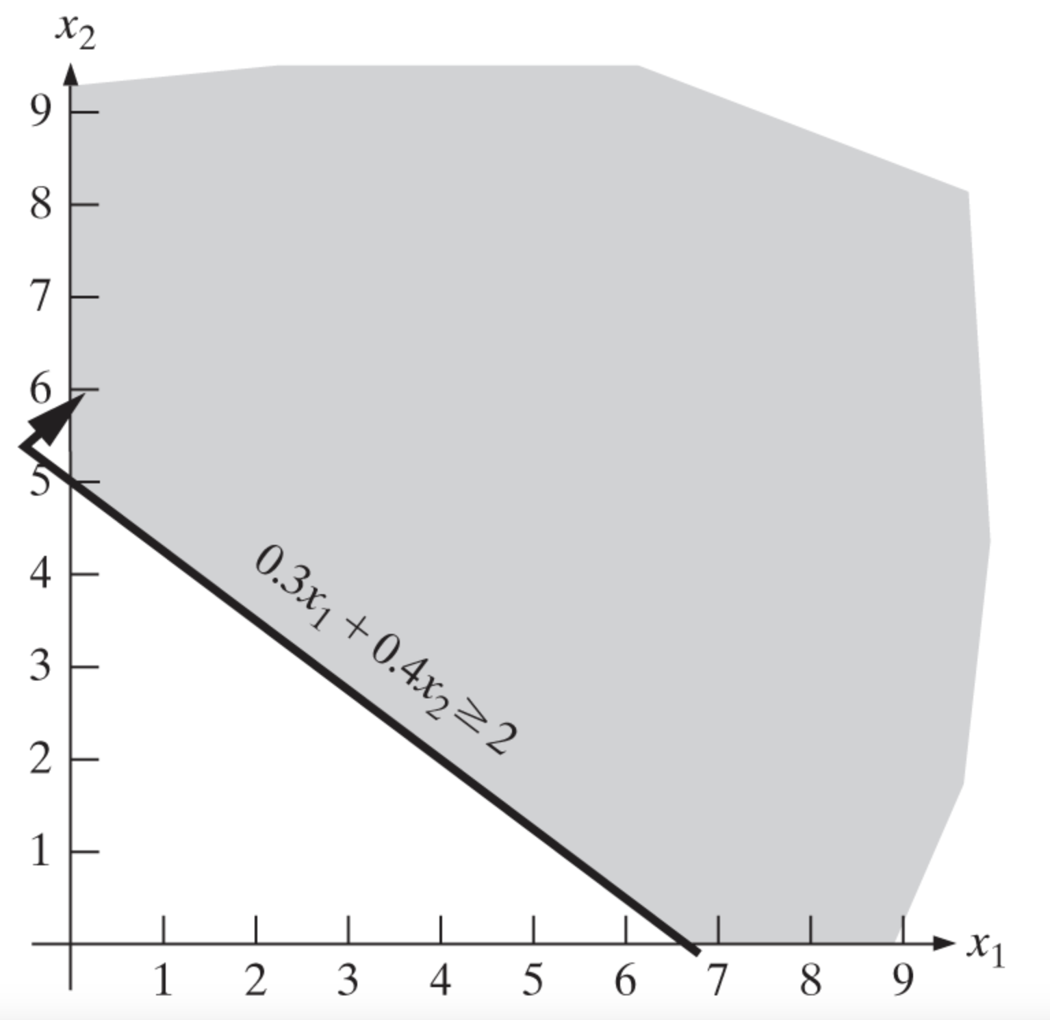
If you wonder how this line is drawn, remember we can pick two points to draw a line. For example, if we pick \(x_1 = 0\) then \(x_2 = 5\) and if we pick \(x_2 = 0\) then \(x_1 = 6.67\). Then, we can draw a line between these two points. That’s the line you see on the plane. As for the direction of the inequality, we can use the point \((0,0)\) to decide which side of the line is feasible. If the point \((0,0)\) satisfies the inequality, then the feasible region is on the same side of the line with the point \((0,0)\). If the point \((0,0)\) does not satisfy the inequality, then the feasible region is on the other side of the line. In our example, the point \((0,0)\) does not satisfy the inequality. Therefore, the feasible region is on the other side of the line.

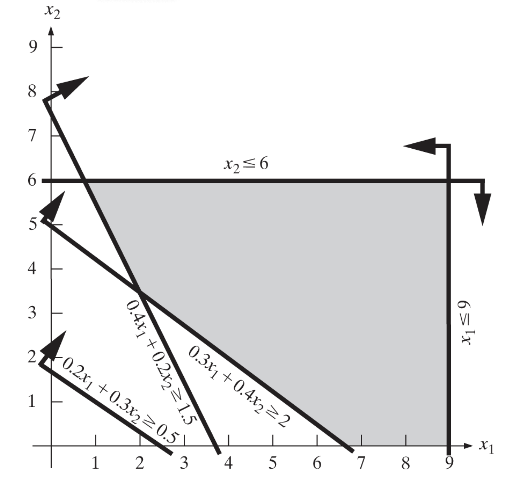
An important observation here is we are using the intersection of three inequalities to define the feasible region. That is, the feasible region is the intersection of the three half-planes. Similarly, we can add the remaining constraints to the current feasible region. The final feasible region is shown in the following figure:

Figure 3: final feasible solution space, all constraints added. Courtesy of reference 1

Now that we know the feasible solution space (any combinations of \(x_1\) and \(x_2\) that is in the feasible region), we can find the optimal solution. The optimal solution is the point that minimizes the objective function (remember our objective is minimization in this case!). In our example, the objective function is \(100x_1 + 75x_2\). We can draw a line for this objective function. The line is shown in the following figure:

Figure 4: objective function is plotted on the solution space. Contours show the possible solutions with the same objective function value. Courtesy of reference 1

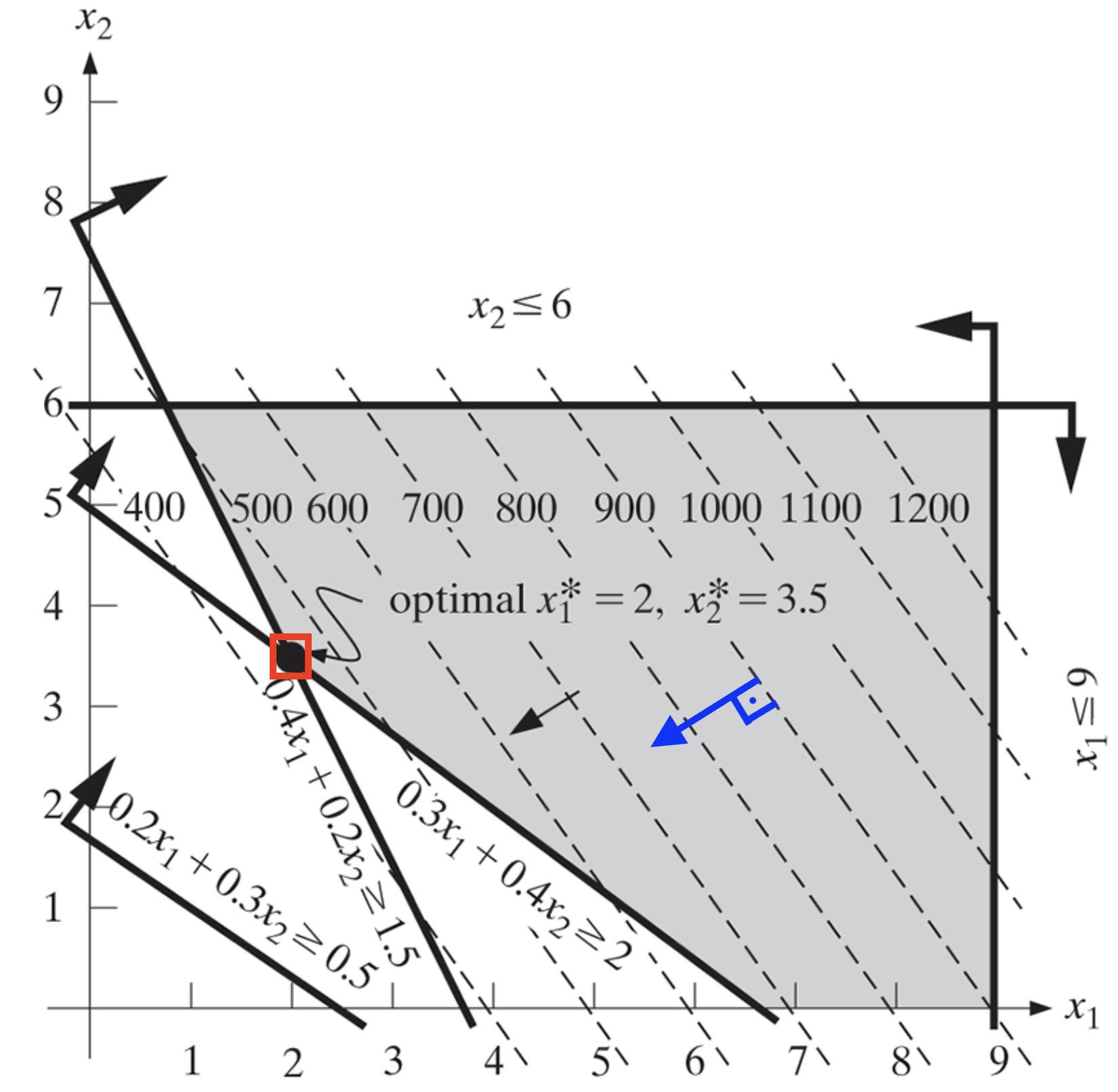
The optimal is the last point before the objective function line leaves the feasible region while moving towards the improving direction-the direction perperdicular to the objective function and make the objective function value smaller and smaller as moved along. In our example, the optimal solution is \((x_1, x_2) = (6, 4)\). The optimal value is \(100x_1 + 75x_2 = 100 \times 6 + 75 \times 4 = 900\). Optimal solution is squred in red and the improving direction is drawn in blue.

An optimization model can have:

• No feasible solution (example 2.6b)
• A unique optimal solution (example 2.5b)
• Multiple optimal solutions (example 2.5a)
• An unbounded model (example 2.7b)

References

1: Optimization in OR textbook by R. Rardin