Machine Learning Integration with Optimization Models

Introduction

The following LP we solved in the class assumed that the parameters are known. However, in practice, the parameters are not known and they are estimated from the data. ML models can be used to estimate the parameters. Let’s estimate \(p_i, d_i,s_i\) from the data and solve the LP. These parameters correspond to the profit, demand, and the percentage of demand met for region \(i\). This application illustrates how machine learning can be used to predict parameters of an optimization model. We predict demands, unit profits, and percentage of demand satisfied for 4 regions. We are using the optimization model of Exercise 4.1.

Demand features (20 features):

• Historical Sales Data: Past sales figures for the product in each region.
• Price: Current and historical prices of the product.
• Promotions: Information on past and current promotions or discounts.
• Seasonality: Time of year, to capture seasonal effects on demand.
• Market Trends: Data on overall market growth or decline.
• Competitor Pricing: Prices of similar products from competitors.
• Consumer Sentiment: Measures of consumer confidence or sentiment indices.
• Economic Indicators: GDP growth rate, unemployment rate, etc.
• Weather Conditions: Especially for products sensitive to weather changes.
• Special Events: Holidays, sports events, or local festivals.
• Product Availability: Stock levels or supply chain issues.
• Marketing Spend: Amount spent on advertising and promotions.
• Online Search Trends: Volume of online searches related to the product.
• Social Media Sentiment: Sentiment analysis of mentions on social media.
• Population Growth: Changes in the population size in each region.
• Income Levels: Average income or economic prosperity in each region.
• Technological Trends: Adoption rates of relevant technologies.
• Legal/Regulatory Changes: Any changes that might affect demand.
• Health and Safety Concerns: For products affected by health trends.
• International Factors: Exchange rates, international trade policies.

Profit features (20 features):

Costs Related Features: Material costs, labor costs, transportation costs, economies of scale, etc.,

Percentage of Demand Satisfied Features (10 features):

Supply Chain Efficiency: Lead time, supplier reliability, production capacity, inventory levels, etc.,

The mathematical programming model is as follows:

\[ \begin{aligned} \text{Maximize} \quad & \sum_{i=1}^{4}p_{i} x_{i} \\ \text{Subject to} \quad & \sum_{i=1}^{4} x_{i} \leq 0.6\sum_{i=1}^{4}d_{i} \\ & x_{i} \geq s_{i}d_{i} \times 0.01 & \text{for } i=1,2,3,4 \\ & x_{i} \leq d_{i} & \text{for } i=1,2,3,4 \\ & x_{i} \geq 0 & \text{for } i=1,2,3,4 \end{aligned} \]

Scikit-learn documentation is one of the best resources for learning about ML.

• Getting Started with ML

In a typical ML pipeline, the following steps are followed: 1. Data Preprocessing 2. Model Building 3. Model Evaluation 4. Model Deployment

Here we will generate random data to use as features and target values. Targets are the parameters of the LP model. We will use the features to estimate the parameters and solve the LP model. The following Python code generates synthetic data for the features and targets. The data is then split into training and testing sets for each target. The features are stored in a DataFrame for easier manipulation and visualization. The code also demonstrates how to use the AMPL API to solve the LP model.

Code

import numpy as np
import pandas as pd
from sklearn.model_selection import train_test_split
from sklearn.preprocessing import StandardScaler
from sklearn.ensemble import RandomForestRegressor, GradientBoostingRegressor
from sklearn.linear_model import Ridge
from sklearn.metrics import mean_squared_error
from sklearn.pipeline import Pipeline
from sklearn.multioutput import MultiOutputRegressor


# Setting a seed for reproducibility
np.random.seed(56)

# Define feature names
demand_features = [f'demand_feature_{i}' for i in range(1, 21)]
profit_features = [f'profit_feature_{i}' for i in range(1, 21)]
demand_satisfied_features = [f'demand_satisfied_feature_{i}' for i in range(1, 11)]

# Combine all feature names (assuming some overlap for conceptual purposes, but here they'll be unique)
all_features = demand_features + profit_features + demand_satisfied_features

# Generate synthetic data for features
num_samples = 100
X_data = np.random.rand(num_samples, 50)  # 50 features for 100 samples

# Creating a DataFrame for features for clearer visualization and manipulation
X_df = pd.DataFrame(X_data, columns=all_features)

# Generate synthetic targets
y_demand = np.random.rand(num_samples, 4) * 100  # Demand for 4 regions
y_profit = np.random.rand(num_samples, 4) * 50  # Profit for 4 regions
y_demand_satisfied = np.random.rand(num_samples, 4) * 100  # Percentage satisfied for 4 regions

# Split the dataset into training and testing sets for each prediction target
X_train, X_test, y_demand_train, y_demand_test = train_test_split(X_df, y_demand, test_size=0.2, random_state=42)
_, _, y_profit_train, y_profit_test = train_test_split(X_df, y_profit, test_size=0.2, random_state=42)
_, _, y_demand_satisfied_train, y_demand_satisfied_test = train_test_split(X_df, y_demand_satisfied, test_size=0.2, random_state=42)


print(f'data frame look like {X_df.head()} \n dimensions are {X_df.shape}')

data frame look like    demand_feature_1  demand_feature_2  demand_feature_3  demand_feature_4  \
0          0.984192          0.333412          0.673702          0.196390   
1          0.967463          0.282314          0.826301          0.372157   
2          0.065982          0.979526          0.895196          0.695328   
3          0.232980          0.970966          0.366370          0.855239   
4          0.058636          0.280632          0.491215          0.087159   

   demand_feature_5  demand_feature_6  demand_feature_7  demand_feature_8  \
0          0.354446          0.813366          0.247850          0.458611   
1          0.468981          0.188388          0.152736          0.001642   
2          0.099584          0.794967          0.656986          0.279109   
3          0.790406          0.030076          0.426081          0.756142   
4          0.844277          0.309369          0.290016          0.731976   

   demand_feature_9  demand_feature_10  ...  demand_satisfied_feature_1  \
0          0.877301           0.391658  ...                    0.585737   
1          0.458621           0.038813  ...                    0.966455   
2          0.083014           0.502967  ...                    0.093087   
3          0.863558           0.183554  ...                    0.111489   
4          0.880688           0.627432  ...                    0.327852   

   demand_satisfied_feature_2  demand_satisfied_feature_3  \
0                    0.156526                    0.786076   
1                    0.206787                    0.515608   
2                    0.901483                    0.871251   
3                    0.186685                    0.533730   
4                    0.139891                    0.324086   

   demand_satisfied_feature_4  demand_satisfied_feature_5  \
0                    0.165338                    0.744338   
1                    0.572276                    0.887209   
2                    0.387255                    0.594047   
3                    0.474820                    0.909879   
4                    0.361859                    0.240684   

   demand_satisfied_feature_6  demand_satisfied_feature_7  \
0                    0.259254                    0.752243   
1                    0.690391                    0.441933   
2                    0.879337                    0.545526   
3                    0.978251                    0.046860   
4                    0.411413                    0.165687   

   demand_satisfied_feature_8  demand_satisfied_feature_9  \
0                    0.128924                    0.025421   
1                    0.723753                    0.061259   
2                    0.678951                    0.342969   
3                    0.040996                    0.981357   
4                    0.761940                    0.735345   

   demand_satisfied_feature_10  
0                     0.176581  
1                     0.033002  
2                     0.289688  
3                     0.467296  
4                     0.988387  

[5 rows x 50 columns] 
 dimensions are (100, 50)

Code

# Pipeline for demand prediction
demand_pipeline = Pipeline([
    ('scaler', StandardScaler()),
    ('regressor', RandomForestRegressor(n_estimators=100, random_state=42))
])

# Pipeline for profit prediction
profit_pipeline = Pipeline([
    ('scaler', StandardScaler()),
    # Wrap the regressor with MultiOutputRegressor
    ('regressor', MultiOutputRegressor(GradientBoostingRegressor(n_estimators=100, random_state=42)))
])

# Pipeline for demand satisfied prediction
demand_satisfied_pipeline = Pipeline([
    ('scaler', StandardScaler()),
    # Wrap the regressor with MultiOutputRegressor
    ('regressor', MultiOutputRegressor(Ridge(alpha=1.0)))
])

# Train each pipeline
demand_pipeline.fit(X_train, y_demand_train)
profit_pipeline.fit(X_train, y_profit_train)
demand_satisfied_pipeline.fit(X_train, y_demand_satisfied_train)

# Making predictions
y_demand_pred = demand_pipeline.predict(X_test)
y_profit_pred = profit_pipeline.predict(X_test)
y_demand_satisfied_pred = demand_satisfied_pipeline.predict(X_test)

# Compile results into a DataFrame
results_df = pd.DataFrame({
    'Region': ['Region 1', 'Region 2', 'Region 3', 'Region 4'],
    'Demand Prediction': y_demand_pred.mean(axis=0),
    'Profit Prediction': y_profit_pred.mean(axis=0),
    'Demand Satisfied Prediction': y_demand_satisfied_pred.mean(axis=0)
})

print(results_df)

     Region  Demand Prediction  Profit Prediction  Demand Satisfied Prediction
0  Region 1          48.074735          26.214470                    29.900298
1  Region 2          44.381077          24.049736                    45.463532
2  Region 3          50.392137          23.973054                    55.957755
3  Region 4          49.058603          23.533582                    47.548125

Code

%pip install -q amplpy matplotlib
from amplpy import AMPL, ampl_notebook
ampl = ampl_notebook(
    modules=["cbc", "highs","gurobi"],  # modules to install
    license_uuid="cf1b53af-8068-4af6-85e2-41060092fde9",  # license to use
)  # instantiate AMPL object and register magics

[notice] A new release of pip is available: 24.0 -> 24.2
[notice] To update, run: /Library/Developer/CommandLineTools/usr/bin/python3 -m pip install --upgrade pip
Note: you may need to restart the kernel to use updated packages.
Licensed to AMPL Community Edition License for <harun.pirim@ndsu.edu>.

/Users/harunpirim/Library/Python/3.9/lib/python/site-packages/urllib3/__init__.py:35: NotOpenSSLWarning: urllib3 v2 only supports OpenSSL 1.1.1+, currently the 'ssl' module is compiled with 'LibreSSL 2.8.3'. See: https://github.com/urllib3/urllib3/issues/3020
  warnings.warn(

Code

%%ampl_eval
reset;
param d{1..4}; # demand
param p{1..4}; # profit
param s{1..4}; # demand satisfied
var x{1..4} >=0; # quantity to produce
maximize z: sum{i in 1..4} p[i]*x[i];
capacity: sum{i in 1..4}x[i]<= 0.6*sum{i in 1..4}d[i];
demand1{i in 1..4}: x[i] >= s[i]*d[i]*0.01;
demand2{i in 1..4}: x[i] <= d[i];

Code

ampl.param["d"] = results_df["Demand Prediction"].values;
ampl.param["p"] = results_df["Profit Prediction"].values;
ampl.param["s"] = results_df["Demand Satisfied Prediction"].values;
ampl.option["solver"] = "cbc";
ampl.solve();

cbc 2.10.10: cbc 2.10.10: optimal solution; objective 2849.019107
0 simplex iterations
 

Code

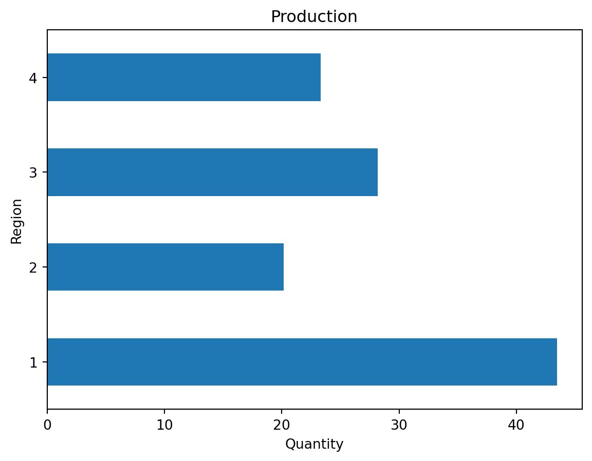
# create a solution report
print(f"Profit = {ampl.obj['z'].value()}")

print("\nProduction Report")
for product, Sell in ampl.var["x"].to_dict().items():
    print(f" For region {product} produced = {Sell}")
#plot the results
production = pd.Series(ampl.var["x"].to_dict())
plot = production.plot(kind="barh", title="Production")
plot.set_xlabel("Quantity")
plot.set_ylabel("Region")

Profit = 2849.0191074318773

Production Report
 For region 1 produced = 43.44197186598346
 For region 2 produced = 20.17720525125885
 For region 3 produced = 28.1983081300234
 For region 4 produced = 23.32644620961024

Text(0, 0.5, 'Region')

References

1: Optimization in OR textbook by R. Rardin