Sensitivity Analysis and Duality

Introduction

In this lecture, we will discuss the sensitivity analysis and duality in linear programming. Sensitivity analysis is the study of how the optimal solution of a linear program changes as the coefficients of the objective function and the right-hand side of the constraints change. Duality is a fundamental concept in linear programming that provides a way to analyze the problem from a different perspective. We will start with sensitivity analysis and then move on to duality.

We cannot solely rely on the optimal solution of the mathematical model that is built with deterministic parameters. In real-world applications, the parameters of the model are not known with certainty. Therefore, it is important to understand how the optimal solution changes as the parameters change. Sensitivity analysis provides a way to understand the impact of changes in the parameters on the optimal solution.

“we will see that there is an entirely separate dual linear program, defined on the same input constants as the main primal model, that has optimal solutions replete with sensitivity insights.” [1]

We will call variables and constraints as generic activities and resources. We will call objective functions as costs or benefits. In order to make sense of the inequalities, we will assume that the right-hand side of the constraints non-negative values.

We will generalize LP constraints as either supply or demand constraints. Supply constraints are the constraints that limit the amount of resources available. Demand constraints are the constraints that limit the amount of resources required. Supply constraints are less than or equal to constraints, and demand constraints are greater than or equal to constraints. Equality constraints can be considered as both supply and demand constraints.

Qualitative Sensitivity Analysis

The image below shows Two Crude example where \(x_1\) is represented as processing activity of Saudi pertoleum in 1000s of barrels, inputs for this activity are left hand-side coefficients of supply constraints (\(\leq\)) and outputs are right hand-side coefficients of demand constraints (\(\geq\)). In other words, supply constraints represent inputs consumed and demand constraints represent outputs produced.

Figure 1: Two Crude example [1]

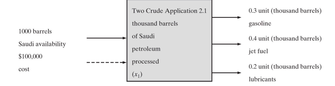
• Each unit (thousand barrels) of Saudi petroleum refined in the Two Crude inputs 1 unit (thousand barrels) of Saudi availability and 100 units (thousand dollars) cost to output 0.3 unit (thousand barrels) of gasoline, 0.4 unit (thousand barrels) of jet fuel, and 0.2 unit (thousand barrels) of lubricants.

See example 6.1

Relaxation vs Tightening of the Solution Space

Figure 2 shows the effects of increasing right-hand side (RHS) of demand constraints on the solution space.

Figure 2: Relaxation vs Tightening of the Solution Space [1]

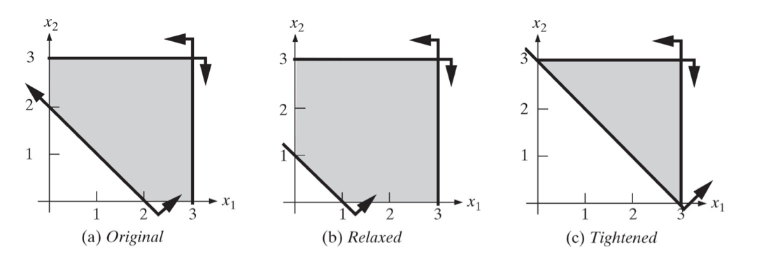
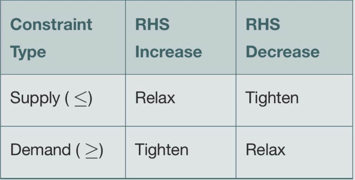
Figure 3 shows general effects of increasing or decreasing the right-hand side of the demand constraints or supply constraints on the solution space.

Figure 3: General Effects of Increasing or Decreasing the Right-Hand Side of the Demand Constraints or Supply Constraints [1]

See example 6.2

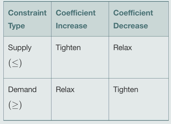
We can discuss changing LSH coefficients of supply and demand constraints. They would have the opposite effect of changing RHS coefficients as seen in Figure 4.

Figure 4: General Effects of Increasing or Decreasing the Left-Hand Side of the Demand Constraints or Supply Constraints [1]

See example 6.3

Adding or Removing Constraints

Adding or removing constraints can change the solution space. Adding constraints can tighten the solution space, and removing constraints can relax the solution space. See example 6.4

Changing the Objective Function Coefficients

Changing the objective function coefficients can change the optimal solution. If the objective function coefficients of the activities are increased (for a maximization problem), the optimal solution will shift towards those activities possibly increasing the optimal value. If the objective function coefficients of the activities are decreased, the optimal solution will shift away from those activities. Figure 5 summarizes the situation.

Figure 5: Changing the Objective Function Coefficients [1]

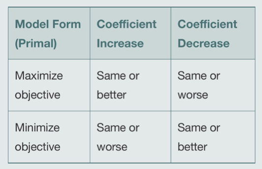
See example 6.6

Adding or Removing Activities (Variables)

Inclusion of activities in the model can change the optimal solution. If an activity is added to the model, the optimal solution may shift towards that activity (possibly improving the objective function value). If an activity is removed from the model, the optimal solution may shift away from that activity (possibly degrading the optimal value). See example 6.8.

Rate of Changes

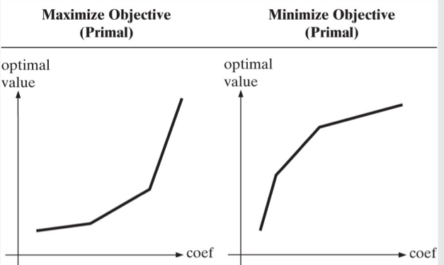
In case the objective function coefficients change improves (increase for maximization, decrease for minimization problems) the optimal value, increasing coefficients more improves the optimal value even more (rate of change (slope) increases). In case of degradation, increasing coefficients more hurts the optimal value less (rate of change decreases). This relationship is illustrated in Figure 6.

Figure 6: Rate of Changes with Objective F. Coefficients [1]

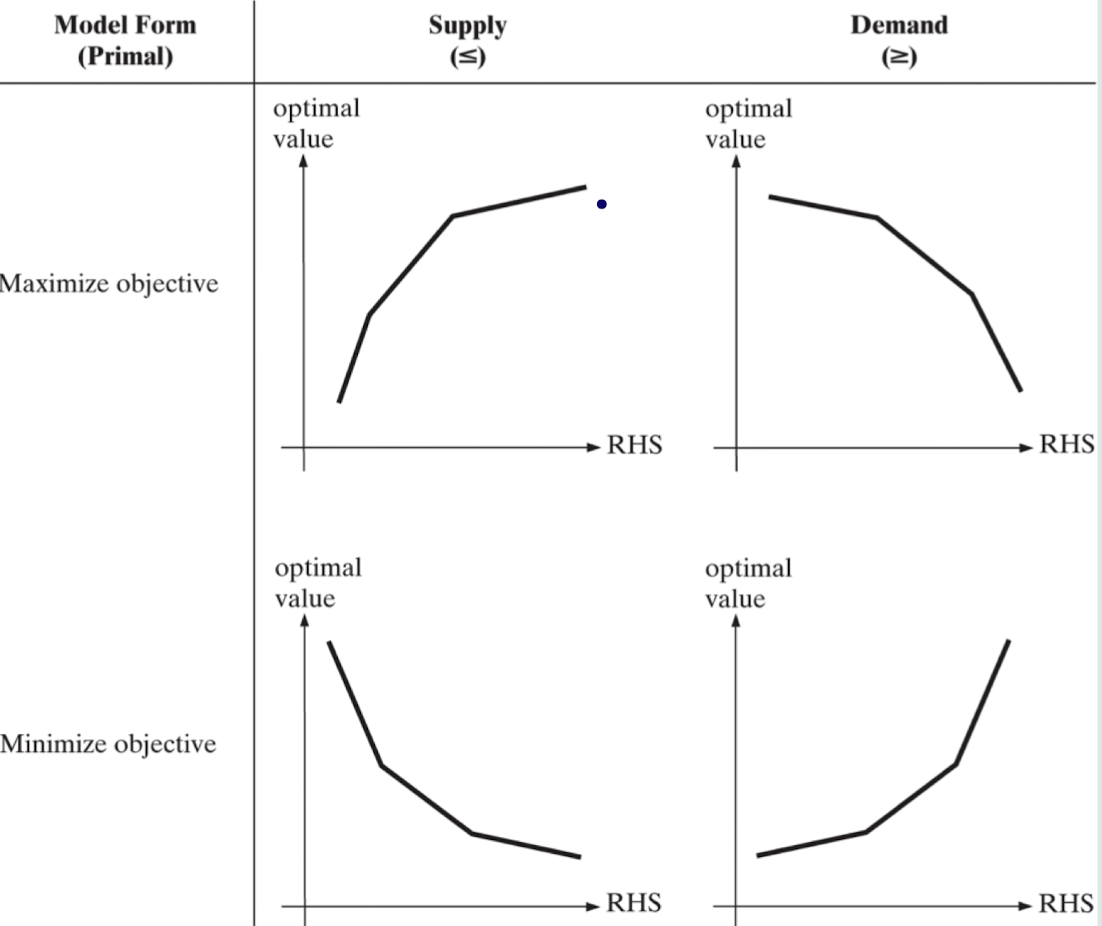
RHS changes have the opposite effect. In case the RHS changes improve the optimal value, increasing RHS more improves the optimal value less (rate of change decreases). In case of degradation, increasing RHS more hurts the optimal value more (rate of change increases). This relationship is illustrated in Figure 7.

Figure 7: Rate of Changes with RHS [1]

References

1: Optimization in OR textbook by R. Rardin